2013年12月15日日曜日
Macにてboost-1.55.0をgcc-4.8.2でコンパイルする。
すでにmacportsを使ってgcc-4.8をインストールしてある。
コマンドラインで使えるgccをgcc-4.8に切り替える。
確認。
boost_1_55_0をダウンロードし解凍する。
ここに移る。
以下を実行。
パスを通す(.bash_profileあるいは.bashrcに記述)。
完了。
2013年11月3日日曜日
opencv-2.4.6.1をApple LLVM version 5.0でコンパイルする
ソースをダウンロードして解凍する。
以下を実行。
こんなエラーが出た。
ここの指摘に従って、
cmakeのオプションに-DBUILD_PERF_TESTS=OFFを追加。
再度、make。今度はこんなエラーが出た。
opencv-2.4.6.1/modules/legacy/src/dpstereo.cppにあるマクロ
が原因である。マクロをinline関数に書き換える。
再度make。今度は上手いく。
完了。
Mac OS X 10.9 Mavericksでport selfupdate
Mac OS X 10.9 Mavericksにしたあと
を実行すると、こんなエラーが出た。
以下を実行。
再度
を実行、今度は無事、MacPorts 2.2.1にアップデートできた。
続けて、
を実行。しばらくするとこれが出た。
サポートしてないとのことなのでこれを実行(llvm-3.0に依存したportsを全てアンインストール)。
再度、
を実行。最後にこれを実行。
完了。
2013年10月3日木曜日
共役な方向とは?
最適化問題の局所的探索法のひとつに共役勾配法がある。この共役な勾配について簡単にまとめる。
いま、最小化すべき関数を$f\left(\vec{x}\right)$とする。$\vec{x}$ 近傍の微小量 $\vec{u}$ と $\vec{v}$ を考え、 $f\left(\vec{x}+\vec{u}+\vec{v}\right)$ を $\vec{x}$ 近傍でTayler展開し、2次の項までとる。 \begin{eqnarray} f\left(\vec{x}+\vec{u}+\vec{v}\right)&=&f\left(\vec{x}\right)+\sum_{i}\frac{\partial f\left(\vec{x}\right)}{\partial x_i}\left(u_i + v_i\right)+\frac{1}{2}\sum_{ij}\frac{\partial^2 f\left(\vec{x}\right)}{\partial x_i \partial x_j}\left(u_i + v_i\right)\left(u_j + v_j\right)\nonumber \\ &=& f\left(\vec{x}\right) + \sum_{i}\frac{\partial f\left(\vec{x}\right)}{\partial x_i}u_i + \frac{1}{2}\sum_{ij}\frac{\partial^2 f\left(\vec{x}\right)}{\partial x_i \partial x_j}u_i\; u_j \nonumber \\ &+& \sum_{i}\frac{\partial f\left(\vec{x}\right)}{\partial x_i}v_i + \frac{1}{2}\sum_{ij}\frac{\partial^2 f\left(\vec{x}\right)}{\partial x_i \partial x_j}v_i\; v_j \nonumber \\ &+& \sum_{ij}\frac{\partial^2 f\left(\vec{x}\right)}{\partial x_i \partial x_j}u_i\;v_j \end{eqnarray} ここで、$b_i=\frac{\partial f}{\partial x_i}$、$A_{ij}=\frac{\partial^2 f}{\partial x_i \partial x_j}$と書くと \begin{equation} \delta f = \left(\vec{b}^{\;T}\vec{u} + \frac{1}{2}\vec{u}^{\;T} A \;\vec{u}\right) +\left(\vec{b}^{\;T}\vec{v} + \frac{1}{2}\vec{v}^{\;T} A \;\vec{v}\right) + \vec{u}^{\;T}\;A\;\vec{v} \end{equation} となる。上式右辺の最後の項が存在しなければ、$\vec{u}$ と $\vec{v}$ について独立に局所的探索法を適用できる。 $\vec{u}^{\;T}\;A\;\vec{v}= 0$ となるような組 $\{\vec{u},\vec{v}\}$ を共役な関係にあるベクトルと呼ぶ。共役な関係にある勾配の集合を適当に作り、互いに干渉することなく効率良く最適解を探索する手法が共役勾配法である。
いま、最小化すべき関数を$f\left(\vec{x}\right)$とする。$\vec{x}$ 近傍の微小量 $\vec{u}$ と $\vec{v}$ を考え、 $f\left(\vec{x}+\vec{u}+\vec{v}\right)$ を $\vec{x}$ 近傍でTayler展開し、2次の項までとる。 \begin{eqnarray} f\left(\vec{x}+\vec{u}+\vec{v}\right)&=&f\left(\vec{x}\right)+\sum_{i}\frac{\partial f\left(\vec{x}\right)}{\partial x_i}\left(u_i + v_i\right)+\frac{1}{2}\sum_{ij}\frac{\partial^2 f\left(\vec{x}\right)}{\partial x_i \partial x_j}\left(u_i + v_i\right)\left(u_j + v_j\right)\nonumber \\ &=& f\left(\vec{x}\right) + \sum_{i}\frac{\partial f\left(\vec{x}\right)}{\partial x_i}u_i + \frac{1}{2}\sum_{ij}\frac{\partial^2 f\left(\vec{x}\right)}{\partial x_i \partial x_j}u_i\; u_j \nonumber \\ &+& \sum_{i}\frac{\partial f\left(\vec{x}\right)}{\partial x_i}v_i + \frac{1}{2}\sum_{ij}\frac{\partial^2 f\left(\vec{x}\right)}{\partial x_i \partial x_j}v_i\; v_j \nonumber \\ &+& \sum_{ij}\frac{\partial^2 f\left(\vec{x}\right)}{\partial x_i \partial x_j}u_i\;v_j \end{eqnarray} ここで、$b_i=\frac{\partial f}{\partial x_i}$、$A_{ij}=\frac{\partial^2 f}{\partial x_i \partial x_j}$と書くと \begin{equation} \delta f = \left(\vec{b}^{\;T}\vec{u} + \frac{1}{2}\vec{u}^{\;T} A \;\vec{u}\right) +\left(\vec{b}^{\;T}\vec{v} + \frac{1}{2}\vec{v}^{\;T} A \;\vec{v}\right) + \vec{u}^{\;T}\;A\;\vec{v} \end{equation} となる。上式右辺の最後の項が存在しなければ、$\vec{u}$ と $\vec{v}$ について独立に局所的探索法を適用できる。 $\vec{u}^{\;T}\;A\;\vec{v}= 0$ となるような組 $\{\vec{u},\vec{v}\}$ を共役な関係にあるベクトルと呼ぶ。共役な関係にある勾配の集合を適当に作り、互いに干渉することなく効率良く最適解を探索する手法が共役勾配法である。
2013年9月15日日曜日
Kinematics 〜 Implementation 〜
in Japanese
In the previous page, I described a brief explanation on the kinematics. Here I show you my implementation of the algorithm of a six-axis-arm system in C++.
A green sphere indicates a target position. When the end point of the arm arrives at it, the target is moved to the next position.
Here is my source code.
A file
Introduction
In the previous page, I described a brief explanation on the kinematics. Here I show you my implementation of the algorithm of a six-axis-arm system in C++.
Demo
Development Environment
- Mac OS X 10.8.4
- Processor:3.06 GHz Intel Core 2 Duo
- Memory:4GB
- Xcode4.6.2 with Apple LLVM 4.2(C++ Language Dialect → C++11, C++ Standard Library → libc++)
- boost-1.54.0(built by Apple LLVM 4.2 compiler)
Source
Here is my source code.
Usage
A file
robot.dat passed as an argument determines a form of the arm system.
The format of the file is expressed in 1.
Using keyboard,
- 'c' starts the program,
- 'b' inverts the movement of the target sphere,
- 'a' restores the movement,
- and
escapestops the program.
References
- OpenGL 3Dグラフィックス入門 第2版 三浦憲二郎 朝倉書店 (In Japanese)
Kinematics 〜 Theory 〜
in Japanese
In this page, I describe a brief explanation on the kinematics used in the robotics. See also the next page as to the implementation of a simple six-axis-arm system in C++.
Let us consider the 3-dimensional homogeneous coordinate system. In the system, the rotation matrices around x, y, and z axises are given by \begin{equation} R_{x}(\theta) = \left( \begin{array}{cccc} 1 & 0 & 0 & 0 \\ 0 & \cos{\theta} & -\sin{\theta} & 0 \\ 0 & \sin{\theta} & \cos{\theta} & 0 \\ 0 & 0 & 0 & 1 \end{array} \right), \end{equation} \begin{equation} R_{y}(\theta) = \left( \begin{array}{cccc} \cos{\theta} & 0 & \sin{\theta} & 0 \\ 0 & 1 & 0 & 0 \\ -\sin{\theta} & 0 & \cos{\theta} & 0 \\ 0 & 0 & 0 & 1 \end{array} \right), \end{equation} and \begin{equation} R_{z}(\theta) = \left( \begin{array}{cccc} \cos{\theta} & -\sin{\theta} & 0 & 0 \\ \sin{\theta} & \cos{\theta} & 0 & 0 \\ 0 & 0 & 1 & 0 \\ 0 & 0 & 0 & 1 \end{array} \right). \end{equation} Moreover, the translation matrix $L(\vec{l})$ with a directional vector $\vec{l}$ is obtained by \begin{equation} L(\vec{l}) = \left( \begin{array}{cccc} 1 & 0 & 0 & l_x \\ 0 & 1 & 0 & l_y \\ 0 & 0 & 1 & l_z \\ 0 & 0 & 0 & 1 \end{array} \right). \end{equation} Suppose that we have an initial state of a three-axis-arm system shown in the below figure. In the figure, $n_i$ and $l_i$ indicate a joint and a length of each component, respectively.
$n_1$ rotates $\theta_1$ in counterclockwise direction around $x$ axis, $n_2$ rotates $\theta_2$ in counterclockwise direction around $y$ axis, and $n_3$ rotates $\theta_3$ in counterclockwise direction around $x$ axis. $\vec{l}_1=(0,0,l_1)$, $\vec{l}_2=(0,0,l_2)$, and $\vec{l}_3=(0,0,l_3)$.
A position vector of an end point $n_4$ takes the form
\begin{equation}
\vec{p}_{4} = R_x(\theta_1) L(\vec{l}_1) R_y(\theta_2) L(\vec{l}_2) R_x(\theta_3) L(\vec{l}_3)
\left(
\begin{array}{c}
0 \\
0 \\
0 \\
1
\end{array}
\right).
\label{sample-case}
\end{equation}
It must be noted that parameters $\theta_i$ and $\vec{l}_i$ are defined in the local coordinate system of the $i$-th joint.
We can expand eq.(\ref{sample-case}) to the case of $n$-axis-arm system as
\begin{equation}
\vec{p} = R_{a_{1}}(\theta_1) L(\vec{l}_1) R_{a_{2}}(\theta_2) L(\vec{l}_2) \cdots R_{a_{n}}(\theta_n) L(\vec{l}_n)
\left(
\begin{array}{c}
0 \\
0 \\
0 \\
1
\end{array}
\right),
\end{equation}
where $a_{i}\in \{x,y,z\}$.
In the figure, $n_i$ and $l_i$ indicate a joint and a length of each component, respectively.
$n_1$ rotates $\theta_1$ in counterclockwise direction around $x$ axis, $n_2$ rotates $\theta_2$ in counterclockwise direction around $y$ axis, and $n_3$ rotates $\theta_3$ in counterclockwise direction around $x$ axis. $\vec{l}_1=(0,0,l_1)$, $\vec{l}_2=(0,0,l_2)$, and $\vec{l}_3=(0,0,l_3)$.
A position vector of an end point $n_4$ takes the form
\begin{equation}
\vec{p}_{4} = R_x(\theta_1) L(\vec{l}_1) R_y(\theta_2) L(\vec{l}_2) R_x(\theta_3) L(\vec{l}_3)
\left(
\begin{array}{c}
0 \\
0 \\
0 \\
1
\end{array}
\right).
\label{sample-case}
\end{equation}
It must be noted that parameters $\theta_i$ and $\vec{l}_i$ are defined in the local coordinate system of the $i$-th joint.
We can expand eq.(\ref{sample-case}) to the case of $n$-axis-arm system as
\begin{equation}
\vec{p} = R_{a_{1}}(\theta_1) L(\vec{l}_1) R_{a_{2}}(\theta_2) L(\vec{l}_2) \cdots R_{a_{n}}(\theta_n) L(\vec{l}_n)
\left(
\begin{array}{c}
0 \\
0 \\
0 \\
1
\end{array}
\right),
\end{equation}
where $a_{i}\in \{x,y,z\}$.
Setting lengths to constant values, the vector $\vec{p}$ becomes a function with $n$ angles in the form \begin{equation} \vec{p}= \vec{f}(\theta_1,\theta_2,\cdots,\theta_n). \end{equation} Its deviation with respect to $\{\theta_1,\theta_2,\cdots,\theta_n\}$ is written as \begin{eqnarray} \delta\vec{p} &=& \vec{f}(\theta_1+\delta\theta_1,\theta_2+\delta\theta_2,\cdots,\theta_n+\delta\theta_n) - \vec{f}(\theta_1,\theta_2,\cdots,\theta_n)\nonumber \\ &=&\sum_{i=1}^{n}\;\frac{\partial\vec{f}}{\partial\theta_i}\;\delta\theta_i + \frac{1}{2}\sum_{i=1}^{n}\sum_{j=1}^{n}\;\frac{\partial^2\vec{f}}{\partial\theta_i\partial\theta_j}\;\delta\theta_i\;\delta\theta_j +\cdots. \end{eqnarray} Ignoring the terms more than first derivative, we can obtain the form \begin{eqnarray} \left( \begin{array}{c} \delta p_x \\ \delta p_y \\ \delta p_z \end{array} \right) &=& \left(\frac{\partial\vec{f}}{\partial\theta_1},\frac{\partial\vec{f}}{\partial\theta_2},\cdots,\frac{\partial\vec{f}}{\partial\theta_n}\right) \left( \begin{array}{c} \delta \theta_1 \\ \delta \theta_2 \\ \vdots \\ \delta \theta_n \end{array} \right) \nonumber \\ &=& \left( \begin{array}{cccc} \frac{\partial f_1}{\partial \theta_1} & \frac{\partial f_1}{\partial \theta_2} & \cdots & \frac{\partial f_1}{\partial \theta_n} \\ \frac{\partial f_2}{\partial \theta_1} & \frac{\partial f_2}{\partial \theta_2} & \cdots & \frac{\partial f_2}{\partial \theta_n} \\ \frac{\partial f_3}{\partial \theta_1} & \frac{\partial f_3}{\partial \theta_2} & \cdots & \frac{\partial f_3}{\partial \theta_n} \end{array} \right) \left( \begin{array}{c} \delta \theta_1 \\ \delta \theta_2 \\ \vdots \\ \delta \theta_n \end{array} \right) \nonumber \\ &\equiv& J \left( \begin{array}{c} \delta \theta_1 \\ \delta \theta_2 \\ \vdots \\ \delta \theta_n \end{array} \right), \end{eqnarray} where $J$ is called the Jacobian matrix. In this case, it is $3 \times n$ matrix. A partial differential $\frac{\partial \vec{f}}{\partial \theta_i}$ is calculated as \begin{equation} \frac{\partial \vec{f}}{\partial \theta_i} = R_{a_{1}}(\theta_1) L(\vec{l}_1) \cdots \frac{dR_{a_{i}}(\theta_i)}{d\theta_i} L(\vec{l}_i) \cdots R_{a_{n}}(\theta_n) L(\vec{l}_n) \left( \begin{array}{c} 0 \\ 0 \\ 0 \\ 1 \end{array} \right). \end{equation} By introducing the inverse matrix $J^{-1}$, we can obtain the deviation vector $\delta \vec{\theta}$ of angles as \begin{equation} \delta \vec{\theta} = J^{-1}\;\delta\vec{p}. \end{equation} When ${\rm rank}(J)>3$, the inverse matrix $J^{-1}$ is not uniquely determined. In other words, in a case where the number of joints are greater than 3, the end position ($\vec{p}$) is achieved by different postures. The typical method to determine a unique posture is to use a pseudoinverse matrix $J^{\#}$ as \begin{equation} \delta \vec{\theta} = J^{\#} \delta\vec{p}, \end{equation} where \begin{equation} J^{\#}=J^{T}\;(J\;J^{T})^{-1}. \end{equation} The procedure to solve the inverse kinematics problem is as follows:
Introduction
In this page, I describe a brief explanation on the kinematics used in the robotics. See also the next page as to the implementation of a simple six-axis-arm system in C++.
Forward Kinematics
Let us consider the 3-dimensional homogeneous coordinate system. In the system, the rotation matrices around x, y, and z axises are given by \begin{equation} R_{x}(\theta) = \left( \begin{array}{cccc} 1 & 0 & 0 & 0 \\ 0 & \cos{\theta} & -\sin{\theta} & 0 \\ 0 & \sin{\theta} & \cos{\theta} & 0 \\ 0 & 0 & 0 & 1 \end{array} \right), \end{equation} \begin{equation} R_{y}(\theta) = \left( \begin{array}{cccc} \cos{\theta} & 0 & \sin{\theta} & 0 \\ 0 & 1 & 0 & 0 \\ -\sin{\theta} & 0 & \cos{\theta} & 0 \\ 0 & 0 & 0 & 1 \end{array} \right), \end{equation} and \begin{equation} R_{z}(\theta) = \left( \begin{array}{cccc} \cos{\theta} & -\sin{\theta} & 0 & 0 \\ \sin{\theta} & \cos{\theta} & 0 & 0 \\ 0 & 0 & 1 & 0 \\ 0 & 0 & 0 & 1 \end{array} \right). \end{equation} Moreover, the translation matrix $L(\vec{l})$ with a directional vector $\vec{l}$ is obtained by \begin{equation} L(\vec{l}) = \left( \begin{array}{cccc} 1 & 0 & 0 & l_x \\ 0 & 1 & 0 & l_y \\ 0 & 0 & 1 & l_z \\ 0 & 0 & 0 & 1 \end{array} \right). \end{equation} Suppose that we have an initial state of a three-axis-arm system shown in the below figure.

Inverse Kinematcis
Setting lengths to constant values, the vector $\vec{p}$ becomes a function with $n$ angles in the form \begin{equation} \vec{p}= \vec{f}(\theta_1,\theta_2,\cdots,\theta_n). \end{equation} Its deviation with respect to $\{\theta_1,\theta_2,\cdots,\theta_n\}$ is written as \begin{eqnarray} \delta\vec{p} &=& \vec{f}(\theta_1+\delta\theta_1,\theta_2+\delta\theta_2,\cdots,\theta_n+\delta\theta_n) - \vec{f}(\theta_1,\theta_2,\cdots,\theta_n)\nonumber \\ &=&\sum_{i=1}^{n}\;\frac{\partial\vec{f}}{\partial\theta_i}\;\delta\theta_i + \frac{1}{2}\sum_{i=1}^{n}\sum_{j=1}^{n}\;\frac{\partial^2\vec{f}}{\partial\theta_i\partial\theta_j}\;\delta\theta_i\;\delta\theta_j +\cdots. \end{eqnarray} Ignoring the terms more than first derivative, we can obtain the form \begin{eqnarray} \left( \begin{array}{c} \delta p_x \\ \delta p_y \\ \delta p_z \end{array} \right) &=& \left(\frac{\partial\vec{f}}{\partial\theta_1},\frac{\partial\vec{f}}{\partial\theta_2},\cdots,\frac{\partial\vec{f}}{\partial\theta_n}\right) \left( \begin{array}{c} \delta \theta_1 \\ \delta \theta_2 \\ \vdots \\ \delta \theta_n \end{array} \right) \nonumber \\ &=& \left( \begin{array}{cccc} \frac{\partial f_1}{\partial \theta_1} & \frac{\partial f_1}{\partial \theta_2} & \cdots & \frac{\partial f_1}{\partial \theta_n} \\ \frac{\partial f_2}{\partial \theta_1} & \frac{\partial f_2}{\partial \theta_2} & \cdots & \frac{\partial f_2}{\partial \theta_n} \\ \frac{\partial f_3}{\partial \theta_1} & \frac{\partial f_3}{\partial \theta_2} & \cdots & \frac{\partial f_3}{\partial \theta_n} \end{array} \right) \left( \begin{array}{c} \delta \theta_1 \\ \delta \theta_2 \\ \vdots \\ \delta \theta_n \end{array} \right) \nonumber \\ &\equiv& J \left( \begin{array}{c} \delta \theta_1 \\ \delta \theta_2 \\ \vdots \\ \delta \theta_n \end{array} \right), \end{eqnarray} where $J$ is called the Jacobian matrix. In this case, it is $3 \times n$ matrix. A partial differential $\frac{\partial \vec{f}}{\partial \theta_i}$ is calculated as \begin{equation} \frac{\partial \vec{f}}{\partial \theta_i} = R_{a_{1}}(\theta_1) L(\vec{l}_1) \cdots \frac{dR_{a_{i}}(\theta_i)}{d\theta_i} L(\vec{l}_i) \cdots R_{a_{n}}(\theta_n) L(\vec{l}_n) \left( \begin{array}{c} 0 \\ 0 \\ 0 \\ 1 \end{array} \right). \end{equation} By introducing the inverse matrix $J^{-1}$, we can obtain the deviation vector $\delta \vec{\theta}$ of angles as \begin{equation} \delta \vec{\theta} = J^{-1}\;\delta\vec{p}. \end{equation} When ${\rm rank}(J)>3$, the inverse matrix $J^{-1}$ is not uniquely determined. In other words, in a case where the number of joints are greater than 3, the end position ($\vec{p}$) is achieved by different postures. The typical method to determine a unique posture is to use a pseudoinverse matrix $J^{\#}$ as \begin{equation} \delta \vec{\theta} = J^{\#} \delta\vec{p}, \end{equation} where \begin{equation} J^{\#}=J^{T}\;(J\;J^{T})^{-1}. \end{equation} The procedure to solve the inverse kinematics problem is as follows:
- Suppose that a target position of the end point is $\vec{p}_{\rm G}$.
- Calculate a displacement $\vec{d} = \vec{p}_{\rm G}-\vec{p}$ where $\vec{p}$ indicates the current positoin of the end point. Using $\vec{d}$, we make a small deviation $\delta \vec{p}=\alpha\;\vec{d}/|\vec{d}|$ where $\alpha$ is an appropriate positive value.
- Using current angles, we calculate $J^{\#}$.
- Calculate $\delta \vec{\theta}=J^{\#} \delta\vec{p}$.
- Update the quantities, $\vec{\theta} \leftarrow \vec{\theta} + \delta \vec{\theta}, \vec{p} \leftarrow \vec{p} + \delta \vec{p}$.
- After updating them, if the displacement $|\vec{d}| = |\vec{p}_{\rm G}-\vec{p}|$ is not in an acceptable error range $\epsilon$, return to 2.
References
- Forward Kinematics (in Japanese)
- Inverse Kinematics by means of Jacobian (in Japanese)
- Kinematics Problem of Robot (in Japanese)
2013年9月7日土曜日
運動学 〜 実装 〜
in English
先のページで解説したアルゴリズムをC++11で実装した。
緑の球が目的の位置を表す。ロボットの手の先がそれに到達すると、球は次の位置へ移動する。
ソースはここ。
引数に渡しているファイルrobot.datによりロボットの形状を決定している。 そのフォーマットは文献1のものを使用した。 キーボードから
はじめに
先のページで解説したアルゴリズムをC++11で実装した。
デモ
開発環境
- Mac OS X 10.8.4
- プロセッサ:3.06 GHz Intel Core 2 Duo
- メモリ:4GB
- Xcode4.6.2 with Apple LLVM 4.2(C++ Language Dialect → C++11, C++ Standard Library → libc++)
- boost-1.54.0(Apple LLVM 4.2でコンパイルしたもの。)
ソース
ソースはここ。
実行方法
引数に渡しているファイルrobot.datによりロボットの形状を決定している。 そのフォーマットは文献1のものを使用した。 キーボードから
- 'c'を入力してスタート
- 'b'を入力すると逆向き
- 'a'を入力すると元の向き
- escapeキーで終了
参考文献
- OpenGL 3Dグラフィックス入門 第2版 三浦憲二郎 朝倉書店
2013年8月23日金曜日
C++メモ 〜 std::regex 〜
大文字小文字を区別せずに検索するには?
出力:
raw string literalを使えばエスケープせずにダブルクオーテーションを利用できる(7行目)。
空白以外の文字列を拾うには? 出力:
数字を拾うには? 出力:
検索文字の先頭と末尾に特定の文字を挿入するには? 出力: 参照
空白以外の文字列を拾うには? 出力:
std::regexのオブジェクトを作る際(10行目)、raw string literalを使えばエスケープを行う必要はない。
数字を拾うには? 出力:
検索文字の先頭と末尾に特定の文字を挿入するには? 出力: 参照
2013年8月6日火曜日
C++メモ 〜 boost::coroutine 〜
Macではlibboost_coroutine.aとlibboost_context.dylib(.a)をリンクする必要があります。
出力:
出力:
出力:
おまけ。 出力:
追記:2014/1/12 ファイルa.txtの内容は以下の通り。 出力: 関数
Routine1のコンストラクタが呼ばれた時点でloop1の中の
yieldが一度呼ばれます。
出力:
loop2の先頭にあるyield(1)が出力の先頭にある1を生成します。
yield(1)がないと、15行目で落ちます。
Routine2のコンストラクタが呼ばれた時点ではAのオブジェクトが設定されていないからです。
出力:
おまけ。 出力:
追記:2014/1/12 ファイルa.txtの内容は以下の通り。 出力: 関数
read_fileのプロトタイプがないと警告がでるようになった(Apple LLVM 5.0, boost-1.55.0)。
2013年8月4日日曜日
運動学
in English
ロボット工学で使われる順運動学と逆運動学についてまとめる。 実装編はこちら。
3次元空間右手系の同次座標で議論を行う。各軸周りの回転行列は以下の通りである。
$x$軸周りの回転行列 $R_{x}(\theta)$:
\begin{equation} R_{x}(\theta) = \left( \begin{array}{cccc} 1 & 0 & 0 & 0 \\ 0 & \cos{\theta} & -\sin{\theta} & 0 \\ 0 & \sin{\theta} & \cos{\theta} & 0 \\ 0 & 0 & 0 & 1 \end{array} \right) \end{equation} $y$軸周りの回転行列 $R_{y}(\theta)$: \begin{equation} R_{y}(\theta) = \left( \begin{array}{cccc} \cos{\theta} & 0 & \sin{\theta} & 0 \\ 0 & 1 & 0 & 0 \\ -\sin{\theta} & 0 & \cos{\theta} & 0 \\ 0 & 0 & 0 & 1 \end{array} \right) \end{equation} $z$軸周りの回転行列 $R_{z}(\theta)$: \begin{equation} R_{z}(\theta) = \left( \begin{array}{cccc} \cos{\theta} & -\sin{\theta} & 0 & 0 \\ \sin{\theta} & \cos{\theta} & 0 & 0 \\ 0 & 0 & 1 & 0 \\ 0 & 0 & 0 & 1 \end{array} \right) \end{equation} また、方向 $\vec{l}$ への並進移動行列 $L(\vec{l})$ は次式で与えられる。 \begin{equation} L(\vec{l}) = \left( \begin{array}{cccc} 1 & 0 & 0 & l_x \\ 0 & 1 & 0 & l_y \\ 0 & 0 & 1 & l_z \\ 0 & 0 & 0 & 1 \end{array} \right) \end{equation} いま各関節 $n_i$ の初期状態が図のように与えられたとする。
関節 $n_1$ は$x$軸周りに $\theta_1$、関節 $n_2$ は$y$軸周りに $\theta_2$、関節 $n_3$ は$x$軸周りに $\theta_3$ だけ回転するとき、端点$n_4$の位置ベクトルは次式で計算される。
\begin{equation}
\vec{p}_{4} = R_x(\theta_1) L(\vec{l}_1) R_y(\theta_2) L(\vec{l}_2) R_x(\theta_3) L(\vec{l}_3)
\left(
\begin{array}{c}
0 \\
0 \\
0 \\
1
\end{array}
\right)
\end{equation}
各関節での局所座標は、その関節に到るまでの変換行列の影響を受ける。回転行列、並進移動行列のパラメータは各関節の局所座標系で定義される量である。一般に関節が$n$個ある場合の端点(end-effector)の位置座標 $\vec{p}$ は
\begin{equation}
\vec{p} = R_{a_{1}}(\theta_1) L(\vec{l}_1) R_{a_{2}}(\theta_2) L(\vec{l}_2) \cdots R_{a_{n}}(\theta_n) L(\vec{l}_n)
\left(
\begin{array}{c}
0 \\
0 \\
0 \\
1
\end{array}
\right)
\end{equation}
となる。ここで$a_{i}\in \{x,y,z\}$である。
腕(リンク)の長さが定数であるとき位置ベクトル $\vec{p}$ は $n$ 個の角度の関数である。 \begin{equation} \vec{p}= \vec{f}(\theta_1,\theta_2,\cdots,\theta_n) \end{equation} 変分をとると \begin{eqnarray} \delta\vec{p} &=& \vec{f}(\theta_1+\delta\theta_1,\theta_2+\delta\theta_2,\cdots,\theta_n+\delta\theta_n) - \vec{f}(\theta_1,\theta_2,\cdots,\theta_n)\nonumber \\ &=&\sum_{i=1}^{n}\;\frac{\partial\vec{f}}{\partial\theta_i}\;\delta\theta_i + \frac{1}{2}\sum_{i=1}^{n}\sum_{j=1}^{n}\;\frac{\partial^2\vec{f}}{\partial\theta_i\partial\theta_j}\;\delta\theta_i\;\delta\theta_j +\cdots \end{eqnarray} 2次以降の項を無視して書き下ろすと \begin{eqnarray} \left( \begin{array}{c} \delta p_x \\ \delta p_y \\ \delta p_z \end{array} \right) &=& \left(\frac{\partial\vec{f}}{\partial\theta_1},\frac{\partial\vec{f}}{\partial\theta_2},\cdots,\frac{\partial\vec{f}}{\partial\theta_n}\right) \left( \begin{array}{c} \delta \theta_1 \\ \delta \theta_2 \\ \vdots \\ \delta \theta_n \end{array} \right) \nonumber \\ &=& \left( \begin{array}{cccc} \frac{\partial f_1}{\partial \theta_1} & \frac{\partial f_1}{\partial \theta_2} & \cdots & \frac{\partial f_1}{\partial \theta_n} \\ \frac{\partial f_2}{\partial \theta_1} & \frac{\partial f_2}{\partial \theta_2} & \cdots & \frac{\partial f_2}{\partial \theta_n} \\ \frac{\partial f_3}{\partial \theta_1} & \frac{\partial f_3}{\partial \theta_2} & \cdots & \frac{\partial f_3}{\partial \theta_n} \end{array} \right) \left( \begin{array}{c} \delta \theta_1 \\ \delta \theta_2 \\ \vdots \\ \delta \theta_n \end{array} \right) \nonumber \\ &\equiv& J \left( \begin{array}{c} \delta \theta_1 \\ \delta \theta_2 \\ \vdots \\ \delta \theta_n \end{array} \right) \end{eqnarray} となる。ここで行列 $J$ はヤコビアン(Jacobian)である。いまの場合 $3 \times n$ の行列となる。要素に現れる偏微分は次式で計算できる。 \begin{equation} \frac{\partial \vec{f}}{\partial \theta_i} = R_{a_{1}}(\theta_1) L(\vec{l}_1) \cdots \frac{dR_{a_{i}}(\theta_i)}{d\theta_i} L(\vec{l}_i) \cdots R_{a_{n}}(\theta_n) L(\vec{l}_n) \left( \begin{array}{c} 0 \\ 0 \\ 0 \\ 1 \end{array} \right) \end{equation} 逆行列 $J^{-1}$を使えば位置の変位量 $\delta \vec{p}$ から角度の変位量 $\delta \vec{\theta}$ を求めることができる。 \begin{equation} \delta \vec{\theta} = J^{-1}\;\delta\vec{p} \end{equation} ${\rm rank}(J)>3$のとき $J$ の逆行列は無数に存在する。 すなわち、関節の数が3より大きい場合、1つの端点(end effector)の位置に対応する腕の姿勢は無数に存在する。したがって、任意の拘束条件を導入して $\delta \vec{\theta}$ を一意に決定する必要がある。その代表的な方法が、擬似逆行列(pseudoinverse)$J^{\#}$ を用いる方法である。 \begin{equation} \delta \vec{\theta} = J^{\#} \delta\vec{p} \end{equation} ここで、 \begin{equation} J^{\#}=J^{T}\;(J\;J^{T})^{-1} \end{equation} である。 逆運動学問題を解く手順は以下の通りである。
はじめに
ロボット工学で使われる順運動学と逆運動学についてまとめる。 実装編はこちら。
順運動学
3次元空間右手系の同次座標で議論を行う。各軸周りの回転行列は以下の通りである。
$x$軸周りの回転行列 $R_{x}(\theta)$:
\begin{equation} R_{x}(\theta) = \left( \begin{array}{cccc} 1 & 0 & 0 & 0 \\ 0 & \cos{\theta} & -\sin{\theta} & 0 \\ 0 & \sin{\theta} & \cos{\theta} & 0 \\ 0 & 0 & 0 & 1 \end{array} \right) \end{equation} $y$軸周りの回転行列 $R_{y}(\theta)$: \begin{equation} R_{y}(\theta) = \left( \begin{array}{cccc} \cos{\theta} & 0 & \sin{\theta} & 0 \\ 0 & 1 & 0 & 0 \\ -\sin{\theta} & 0 & \cos{\theta} & 0 \\ 0 & 0 & 0 & 1 \end{array} \right) \end{equation} $z$軸周りの回転行列 $R_{z}(\theta)$: \begin{equation} R_{z}(\theta) = \left( \begin{array}{cccc} \cos{\theta} & -\sin{\theta} & 0 & 0 \\ \sin{\theta} & \cos{\theta} & 0 & 0 \\ 0 & 0 & 1 & 0 \\ 0 & 0 & 0 & 1 \end{array} \right) \end{equation} また、方向 $\vec{l}$ への並進移動行列 $L(\vec{l})$ は次式で与えられる。 \begin{equation} L(\vec{l}) = \left( \begin{array}{cccc} 1 & 0 & 0 & l_x \\ 0 & 1 & 0 & l_y \\ 0 & 0 & 1 & l_z \\ 0 & 0 & 0 & 1 \end{array} \right) \end{equation} いま各関節 $n_i$ の初期状態が図のように与えられたとする。
逆運動学
腕(リンク)の長さが定数であるとき位置ベクトル $\vec{p}$ は $n$ 個の角度の関数である。 \begin{equation} \vec{p}= \vec{f}(\theta_1,\theta_2,\cdots,\theta_n) \end{equation} 変分をとると \begin{eqnarray} \delta\vec{p} &=& \vec{f}(\theta_1+\delta\theta_1,\theta_2+\delta\theta_2,\cdots,\theta_n+\delta\theta_n) - \vec{f}(\theta_1,\theta_2,\cdots,\theta_n)\nonumber \\ &=&\sum_{i=1}^{n}\;\frac{\partial\vec{f}}{\partial\theta_i}\;\delta\theta_i + \frac{1}{2}\sum_{i=1}^{n}\sum_{j=1}^{n}\;\frac{\partial^2\vec{f}}{\partial\theta_i\partial\theta_j}\;\delta\theta_i\;\delta\theta_j +\cdots \end{eqnarray} 2次以降の項を無視して書き下ろすと \begin{eqnarray} \left( \begin{array}{c} \delta p_x \\ \delta p_y \\ \delta p_z \end{array} \right) &=& \left(\frac{\partial\vec{f}}{\partial\theta_1},\frac{\partial\vec{f}}{\partial\theta_2},\cdots,\frac{\partial\vec{f}}{\partial\theta_n}\right) \left( \begin{array}{c} \delta \theta_1 \\ \delta \theta_2 \\ \vdots \\ \delta \theta_n \end{array} \right) \nonumber \\ &=& \left( \begin{array}{cccc} \frac{\partial f_1}{\partial \theta_1} & \frac{\partial f_1}{\partial \theta_2} & \cdots & \frac{\partial f_1}{\partial \theta_n} \\ \frac{\partial f_2}{\partial \theta_1} & \frac{\partial f_2}{\partial \theta_2} & \cdots & \frac{\partial f_2}{\partial \theta_n} \\ \frac{\partial f_3}{\partial \theta_1} & \frac{\partial f_3}{\partial \theta_2} & \cdots & \frac{\partial f_3}{\partial \theta_n} \end{array} \right) \left( \begin{array}{c} \delta \theta_1 \\ \delta \theta_2 \\ \vdots \\ \delta \theta_n \end{array} \right) \nonumber \\ &\equiv& J \left( \begin{array}{c} \delta \theta_1 \\ \delta \theta_2 \\ \vdots \\ \delta \theta_n \end{array} \right) \end{eqnarray} となる。ここで行列 $J$ はヤコビアン(Jacobian)である。いまの場合 $3 \times n$ の行列となる。要素に現れる偏微分は次式で計算できる。 \begin{equation} \frac{\partial \vec{f}}{\partial \theta_i} = R_{a_{1}}(\theta_1) L(\vec{l}_1) \cdots \frac{dR_{a_{i}}(\theta_i)}{d\theta_i} L(\vec{l}_i) \cdots R_{a_{n}}(\theta_n) L(\vec{l}_n) \left( \begin{array}{c} 0 \\ 0 \\ 0 \\ 1 \end{array} \right) \end{equation} 逆行列 $J^{-1}$を使えば位置の変位量 $\delta \vec{p}$ から角度の変位量 $\delta \vec{\theta}$ を求めることができる。 \begin{equation} \delta \vec{\theta} = J^{-1}\;\delta\vec{p} \end{equation} ${\rm rank}(J)>3$のとき $J$ の逆行列は無数に存在する。 すなわち、関節の数が3より大きい場合、1つの端点(end effector)の位置に対応する腕の姿勢は無数に存在する。したがって、任意の拘束条件を導入して $\delta \vec{\theta}$ を一意に決定する必要がある。その代表的な方法が、擬似逆行列(pseudoinverse)$J^{\#}$ を用いる方法である。 \begin{equation} \delta \vec{\theta} = J^{\#} \delta\vec{p} \end{equation} ここで、 \begin{equation} J^{\#}=J^{T}\;(J\;J^{T})^{-1} \end{equation} である。 逆運動学問題を解く手順は以下の通りである。
- 端点の目標位置を $\vec{p}_{\rm G}$ とする。
- 現在の端点の位置 $\vec{p}$ からの変位量 $\vec{d} = \vec{p}_{\rm G}-\vec{p}$ から微小変位量を求める。$\delta \vec{p}=\alpha\;\vec{d}/|\vec{d}|$。ここで $\alpha$ は適当な微小量である。
- 現在の $\vec{\theta}$ を使って $J^{\#}$ を計算する。
- $\delta \vec{\theta}=J^{\#} \delta\vec{p}$ を計算する。
- $\vec{\theta} \leftarrow \vec{\theta} + \delta \vec{\theta}, \vec{p} \leftarrow \vec{p} + \delta \vec{p}$
- 更新後の変位量 $|\vec{d}| = |\vec{p}_{\rm G}-\vec{p}|$が許容誤差 $\epsilon$ 以下なら計算終了。そうでなければ、2へ戻る。
参考文献
2013年7月5日金曜日
How to build Boost-1.53.0 by Apple LLVM version 4.2 comiler
in Japanese
First install the Command Line Tools of Xcode-4.6.1 and check the version. Download and decompress the boost-1.53.0. Run the following commands: When using it on the Xcode, we need to add a variable
First install the Command Line Tools of Xcode-4.6.1 and check the version. Download and decompress the boost-1.53.0. Run the following commands: When using it on the Xcode, we need to add a variable
DYLD_LIBRARY to "Product→Edit Scheme→Arguments→Environment Variables" and set the path to dylib to the variable.
2013年7月4日木曜日
Computational Geometry
〜 Theory and Practice on the 2D Convex Hull 〜
in Japanese
Input: A sequence of points, $A=\{P_1,P_2,\cdots,P_n\}$ (We call the suffixes the original numbers)
Output: Convex Hull, $C(A)$

Let us turn to the algorithm $X$.
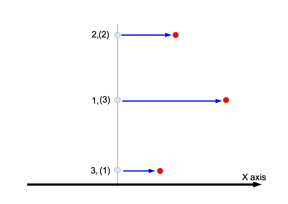
Input:$C(\{P_{(1)},P_{(2)}, \cdots,P_{(k)}\})$, $P_{(k+1)}$, $V_{\rm clockwise}$, $V_{\rm counterclockwise}$, $T_{{\rm sorted}\rightarrow{\rm original}}$
Output:$C(\{P_{(1)},P_{(2)},\cdots,P_{(k+1)}\})$, $V_{\rm clockwise}$, $V_{\rm counterclockwise}$
In order to determine if the path turns left or right, the determinant $F$ as shown in the previous page is used.

Introduction
In this page, I describe a brief explanation on the algorithm of the 2-dimensional convex hull upon which I touched in the previous page. I also show you my implementation of it in C++.Algorithm
The algorithm discussed here is called the Incremental Method which has the complexity of $O(n\log{n})$ 1.Input: A sequence of points, $A=\{P_1,P_2,\cdots,P_n\}$ (We call the suffixes the original numbers)
Output: Convex Hull, $C(A)$
- Arrange points in ascending order of $x$-coordinate values. We write the resultant sequence as $A^{\prime}=\{P_{(1)},P_{(2)},\cdots,P_{(n)}\}$ and call the suffixes the sorted numbers. When two points have the same $x$-coordinate value, we arrange them in descending order of the original numbers. We store the table $T_{{\rm sorted}\rightarrow{\rm original}}$ that maps the sorted number to the original one.
- Make a triangle consisting of the first three points of $A^{\prime}$ and write it as $C(\{P_{(1)},P_{(2)},P_{(3)}\})$. Store two arrays $V_{\rm clockwise}$ and $V_{\rm counterclockwise}$ that allow us to follow points in clockwise order and counterclockwise order, respectively. For instance, if the sorted number $a$ is followed by $b$ when we trace the points in clockwise order, $V_{\rm clockwise}(a)=b$ holds.
- Add points sequentially from $(3)$ to $(n)$. Every time a point is inserted, the algorithm $X$ that is discussed later is executed.
- Finally we obtain the output $C(\{P_{(1)},P_{(2)},\cdots,P_{(n)}\})$. The sequence of points obtained by $V_{\rm clockwise}$ or $V_{\rm counterclockwise}$ provides the convex hull to us.
Let us turn to the algorithm $X$.
Input:$C(\{P_{(1)},P_{(2)}, \cdots,P_{(k)}\})$, $P_{(k+1)}$, $V_{\rm clockwise}$, $V_{\rm counterclockwise}$, $T_{{\rm sorted}\rightarrow{\rm original}}$
Output:$C(\{P_{(1)},P_{(2)},\cdots,P_{(k+1)}\})$, $V_{\rm clockwise}$, $V_{\rm counterclockwise}$
- $P_{(s)}\leftarrow P_{(k)}$
- Consider three points, $P_{(k+1)}$, $P_{(s)}$, and $P_{(t)}$, where $t=V_{\rm counterclockwise}(s)$.
- Trace these points in this order. If the path turns right at $P_{(s)}$, return to step 2 after setting $s\leftarrow t$. Otherwise return to step 4. See the figure below.
- Store the sorted number $(u)$ of the point at which the path turns left.
- $P_{(s)}\leftarrow P_{(k)}$
- Consider three points, $P_{(k+1)}$, $P_{(s)}$, and $P_{(t)}$, where $t=V_{\rm clockwise}(s)$.
- Trace these points in this order. If the path turns left at $P_{(s)}$, return to step 6 after setting $s\leftarrow t$. Otherwise return to step 8.
- Store the sorted number $(l)$ of the point at which the path turns right.
- Set $V_{\rm counterclockwise}(l)=k+1$ and $V_{\rm counterclockwise}(k+1)=u$.
- Set $V_{\rm clockwise}(u)=k+1$ and $V_{\rm clockwise}(k+1)=l$.

In order to determine if the path turns left or right, the determinant $F$ as shown in the previous page is used.
- Consider $F(P_{(i)},P_{(j)},P_{(k)})$.
- Convert the sorted numbers to the original ones using $T_{{\rm sorted}\rightarrow{\rm original}}$. \begin{eqnarray} a&=&T_{{\rm sorted}\rightarrow{\rm original}}(i) \nonumber \\ b&=&T_{{\rm sorted}\rightarrow{\rm original}}(j) \nonumber \\ c&=&T_{{\rm sorted}\rightarrow{\rm original}}(k) \nonumber \end{eqnarray}
- Arrange the elements of the list $L=(a,b,c)$ in descending order to generate a new list $L^{\prime}=(a^{\prime},b^{\prime},c^{\prime})$. If the conversion is done with an odd permutation, $p=-1$. Otherwise $p=1$.
- Calculate the value of $F(P_{a^{\prime}},P_{b^{\prime}},P_{c^{\prime}})$. Multiply its sign by $p$ to obtain the sign of $F(P_{a},P_{b},P_{c})$. If it is positive, the path turns left, otherwise turns right.
Implementation in C++
Here is my source code.The functionmain is as follows:
- the 16th-39th lines: The input points are randomly generated.
- the 43th line: An object of the template class
ConvexHull2dis created. In this sample, the type ofintis passed to the template argument. It is also possible to pass the type ofboost::multiprecision::cpp_intto the template argument. - the 44th line: The algorithm is executed.
- after the 46th line: The input points and the convex hull are drawn.
- the 57th line: The sequence of points which constitutes the convex hull is extracted.
Demos


Development Environment
- Mac OS X 10.8.4
- Processor:3.06 GHz Intel Core 2 Duo
- Memory:4GB
- Xcode4.6.2 with Apple LLVM 4.2(C++ Language Dialect → C++11, C++ Standard Library → libc++)
- boost-1.53.0 built by Apple LLVM 4.2 (See here)
- opencv-2.4.5 built by Apple LLVM 4.2 (See here)
Reference
- 計算幾何プログラミング, 杉原厚吉, 岩波書店 (in Japanese)
2013年6月29日土曜日
Windows メモ ~ Dllの作り方 ~
はじめに
Visual StudioにてDllを作成する方法は2つある。
- declspec(dllexport)を使う方法
- declspec(dllexport)を使わない方法
declspec(dllexport)を使う方法
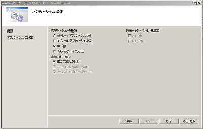
- Win32コンソールアプリケーションを選択。

- アプリケーションの設定で、「DLL」と「空のプロジェクト」を選択。
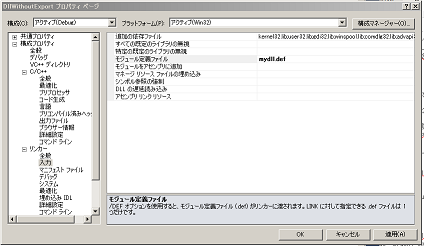
- mydll.hを作成し、以下を記述する。
マクロはプロパティに記述されているものを使うと便利である。ここではDLLWITHEXPORT_EXPORTSを用いた。
そうでない場合は、下記の.cppの一番先頭(#include "mydll.h"の前)にそのマクロを
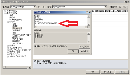
#defineすること。 Dllをビルドする場合は__declspec(dllexport)が使われ、ヘッダとして公開される場合は__declspec(dllimport)が使われる。 - mydll.cppを作成し、以下を記述する。
- ビルドする。DebugあるいはReleaseフォルダ内にプロジェクト名と同じ名前の.lib/.dllファイルが作成される。
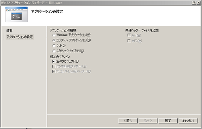
- できあがったDllを使うため、通常のコンソールアプリを作る。
main.cppを作り、以下を記述する。 「追加のインクルードディレクトリ」にmydll.hへのパス、「追加のライブラリディレクトリ」にDllWithExport.libへのパスを記述する。「追加の依存ファイル」にDllWithExport.libを記述する。DllWithExport.dllを実行ファイルと同じフォルダにコピーするか、VSの検索パスに登録しておく(たとえば環境変数に、dllを含むフォルダへのパスを記入する)。 - 実行する。


declspec(dllexport)を使わない方法
- 先と同じようにDll用のプロジェクトを作る。
-
mydll.hを作成し、以下を記述する。
__declspec(dllexport)がないことに注意。 - cppと同じフォルダ内に
mydll.defを作成し、以下を記述する。LIBRARYと同じ行にdll名(プロジェクト名と同じ名前のdll)を、EXPORTSの下に一行ずつexportする関数名を書く。これがdllexportの役割を果たす。 - プロパティの「モジュール定義ファイル」にmydll.defを記述する。
- ビルドする。

C#からの呼び出し
- 空のプロジェクトを作る。
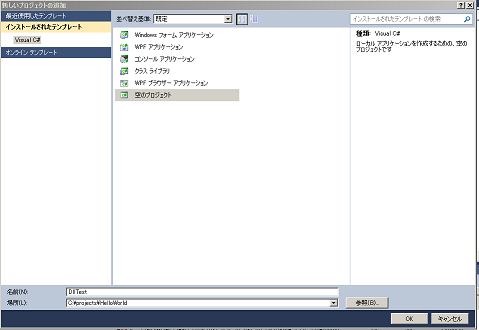
- DllTest.csファイルを作り以下を記述する。
8,9行目でdllから関数
addを取り出し、Addという名前の関数を定義している。 同じ名前のまま使用するなら、EntryPointの記述は必要ない。 - 実行すると失敗する。 「DLL 'DllWithExport.dll'の'add'というエントリポイントが見つかりません」
- dllを作成する際、以下を記述した。 このとき、C++のコンパイラは関数の名前を装飾する。したがって、dllから明示的に関数を取り出す場合、その装飾された名前を指定しなければならない。これを避けるには、Dllを作るとき名前装飾が起こらないようにすればよい。 以下のようにする。 つまり、Cの規約にしたがって関数名を作成する。
- これで実行できる。
- C++のdoubleとC#のdoubleは自動的に対応付けられる。明示的に対応付けが必要な場合はMarshallingなる機能を使う。

2013年6月26日水曜日
Computational Geometry 〜 Symbolic Perturbation 〜
in Japanese

 where points after perturbations are colored in red, and the path $P_i \rightarrow P_j \rightarrow P_k$ after resolving the degeneracy in blue. The detail procedures to (a), (b), and (c) are as follows:
 In this case, the 1st to 7th terms in the right-hand side of eq.(\ref{epsilon_f}) are all zero. The 8th term is the contribution of the perturbation to $y_k$.
Since $\epsilon^{M^{j}}-\epsilon^{M^{i}}>0$, the sign of the 8th term is positive. Therefore, $F(P_i^{\ast},P_j^{\ast},P_k^{\ast})>0$, so the path turns left at $P_j$.
In this case, the 1st to 7th terms in the right-hand side of eq.(\ref{epsilon_f}) are all zero. The 8th term is the contribution of the perturbation to $y_k$.
Since $\epsilon^{M^{j}}-\epsilon^{M^{i}}>0$, the sign of the 8th term is positive. Therefore, $F(P_i^{\ast},P_j^{\ast},P_k^{\ast})>0$, so the path turns left at $P_j$.
From the discussions stated above, the symbolic perturbation method turns out to be the powerful tool to resolve the degeneracies.
Introduction
In the implementation of computational geometry algorithms, it is important to allow numerical calculation to precisely determine the geometric phase structure which depends on the sign of a function $f$. To make the precise judgement, we should use a multiple-precision integer rather than a floating point number in numerical calculation. If floating-point coordinates are given as an input to the algorithm, they just have to be multiplied by a large number and converted to approximated integers. Even if we employ the multiple-precision integer, however, it is impossible to determine the geometric phase structure when ${\rm sign}(f)=0$. The state is called a degeneracy, which occurs when some coordinate values are coincident with each other. It is the symbolic perturbation method that addresses it. In this page, we would like to describe a brief explanation on the method based on the book.Degeneracy
In this explanation, we consider the following determinant: \begin{equation} F(P_i,P_j,P_k) = \left| \begin{array}{ccc} 1 & x_i & y_i \\ 1 & x_j & y_j \\ 1 & x_k & y_k \end{array} \right| \end{equation} where $P_i=(x_i,y_i)$, $P_j=(x_j,y_j)$, and $P_k=(x_k,y_k)$. In the case of a right-hand coordinate system, the determinant is used as follows: The judgement, for example, is used to implement the 2-dimensional convex hull algorithm as shown here. The degeneracy in the judgement occurs when $F(P_i,P_j,P_k) = 0$. In other words, there exists the point $P_k$ on the line through points $P_i$ and $P_j$ as shown below:
Symbolic Perturbation
Suppose that the total number of points is $n$. We consider three points of them under the assumption that $i>j>k$. The perturbation is added to each point as follows: \begin{eqnarray} P_i^{\ast}&=&(x_i+\epsilon^{M^i},y_i+\epsilon^{M^{n+i}}) \nonumber \\ &\equiv&(x_i^{\ast},y_i^{\ast}) \end{eqnarray} where $M$ is a large integer and $\epsilon$ is a minutely small quantity. Because we assume $i>j>k$, the sequence of $\{y_i,y_j,y_k,x_i,x_j,x_k\}$ has an ascending order of perturbation amounts. The symbolic perturbation resolves the degeneracies by taking the following steps:- The coordinate value with the largest deviation, that is $x_k$ in the current example, is shifted. Then we trace the path $P_i \rightarrow P_j \rightarrow P_k^{\ast}$.
- If we still have the degeneracy, the coordinate value with the second largest deviation, that is $x_j$ in the current example, is shifted. Then we trace the path $P_i \rightarrow P_j^{\ast} \rightarrow P_k^{\ast}$.
- The same process is repeated until the degeneracy disappears.

- Only shifting $x_k$, the degeneracy is resolved.
- The degeneracy is not resolved by merely shifting $x_k$. The coordinate with the second largest deviation, $x_j$, also must be shifted to resolve the degeneracy.
- Since the values, $x_i$, $x_j$, and $x_k$ exist along the $x$ axis, the shifting them does not result in the resolution of the degeneracies. The resolution is achieved only when the coordinate with the next largest deviation, $y_k$, is shifted.
- The 1st term in the right-hand side is 0. The 2nd term ($\epsilon^{M^{k}}$'s term) resolves the degeneracy. Since the term has the negative sign, $F(P_i^{\ast},P_j^{\ast},P_k^{\ast})<0$. Therefore, the path turns right at $P_j$.
- The 1st and 2nd terms in the right-hand side are 0. The contribution of the 3rd term ($\epsilon^{M^{j}}$'s term) resolves the degeneracy. Since the sign of the term is negative, $F(P_i^{\ast},P_j^{\ast},P_k^{\ast})<0$. Therefore, the path turns right at $P_j$.
- The 1st to 4th terms in the right-hand side are all 0. The 5th term ($\epsilon^{M^{n+k}}$'s term) resolves the degeneracy. Since the term has the positive sign, $F(P_i^{\ast},P_j^{\ast},P_k^{\ast})>0$. Therefore, the path turns left at $P_j$.

From the discussions stated above, the symbolic perturbation method turns out to be the powerful tool to resolve the degeneracies.
Reference
- 計算幾何プログラミング, 杉原厚吉, 岩波書店 (written in Japanese)
2013年6月17日月曜日
計算幾何 〜 2次元凸包 理論と実践 〜
in English
入力:$A=\{P_1,P_2,\cdots,P_n\}$(添字を固有番号と呼ぶことにする)
出力:凸包 $C(A)$
次にアルゴリズム $X$ について述べる。
入力:$C(\{P_{(1)},P_{(2)},\cdots,P_{(k)}\})$、$P_{(k+1)}$、$V_{\rm clockwise}$、$V_{\rm counterclockwise}$、$T_{{\rm sorted}\rightarrow{\rm original}}$
出力:$C(\{P_{(1)},P_{(2)},\cdots,P_{(k+1)}\})$
右に曲がる、左に曲がるという判定は先のページで取り上げた判定式 $F$ を使えば良い。
はじめに
前回すこしふれた2次元凸包アルゴリズムについて説明し、C++による実装例を示す。アルゴリズム
今回紹介するアルゴリズムは逐次添加法と呼ばれ、$O(n\log{n})$の計算量を持つ1。入力:$A=\{P_1,P_2,\cdots,P_n\}$(添字を固有番号と呼ぶことにする)
出力:凸包 $C(A)$
- $A$に属する点を $x$ 座標の小さい順にならべる。この点列を $A^{\prime}=\{P_{(1)},P_{(2)},\cdots,P_{(n)}\}$ と書き、添字を整列番号と呼ぶことにする。$x$ 座標が同じ値を持つ場合は固有番号の大きいものから並べる。整列番号から固有番号へ変換するテーブル $T_{{\rm sorted}\rightarrow{\rm original}}$ を保持しておく。
- $A^{\prime}$ の最初の3点から三角形を作り、これを $C(\{P_{(1)},P_{(2)},P_{(3)}\})$ とする。時計回りにたどるときの点列 $V_{\rm clockwise}$ と反時計回りにたどるときの点列 $V_{\rm counterclockwise}$ を保持する。たとえば、時計回りにまわったとき整列番号 $a$ の次に整列番号 $b$ の点がくるなら$V_{\rm clockwise}(a)=b$となるようにすればよい。
- 整列番号 $(3)$ から $(n)$ までの点を順に追加する。各点の追加ごとにアルゴリズム $X$(後述)を実行する。
- 出力値 $C(\{P_{(1)},P_{(2)},\cdots,P_{(n)}\})$ を得る。$V_{\rm clockwise}$ あるいは $V_{\rm counterclockwise}$ をたどれば、凸包を得ることができる。
次にアルゴリズム $X$ について述べる。
入力:$C(\{P_{(1)},P_{(2)},\cdots,P_{(k)}\})$、$P_{(k+1)}$、$V_{\rm clockwise}$、$V_{\rm counterclockwise}$、$T_{{\rm sorted}\rightarrow{\rm original}}$
出力:$C(\{P_{(1)},P_{(2)},\cdots,P_{(k+1)}\})$
- $P_{(s)}\leftarrow P_{(k)}$
- 3点 $P_{(k+1)},P_{(s)},P_{(t)}$ を考える。ここで、$t=V_{\rm counterclockwise}(s)$である。
- 3点をこの順にたどったとき右に曲がるなら $s\leftarrow t$ として2へ、左に曲がるなら4へ(下図参照)。
- 左に曲がった整列番号$(u)$を保持する。
- $P_{(s)}\leftarrow P_{(k)}$
- 3点 $P_{(k+1)},P_{(s)},P_{(t)}$ を考える。ここで、$t=V_{\rm clockwise}(s)$である。
- 3点をこの順にたどったとき左に曲がるなら $s\leftarrow t$ として6へ、右に曲がるな8へ。
- 右に曲がった整列番号$(l)$を保持する。
- $V_{\rm counterclockwise}(l)=k+1$、$V_{\rm counterclockwise}(k+1)=u$ とする。
- $V_{\rm clockwise}(u)=k+1$、$V_{\rm clockwise}(k+1)=l$ とする。
右に曲がる、左に曲がるという判定は先のページで取り上げた判定式 $F$ を使えば良い。
- $F(P_{(i)},P_{(j)},P_{(k)})$ を考える。
- $T_{{\rm sorted}\rightarrow{\rm original}}$ を使って、整列番号を固有番号に変換する。 \begin{eqnarray} a&=&T_{{\rm sorted}\rightarrow{\rm original}}(i) \nonumber \\ b&=&T_{{\rm sorted}\rightarrow{\rm original}}(j) \nonumber \\ c&=&T_{{\rm sorted}\rightarrow{\rm original}}(k) \nonumber \end{eqnarray}
- 固有番号のリスト $L=(a,b,c)$ を大きい順に並べ替え、リスト $L^{\prime}=(a^{\prime},b^{\prime},c^{\prime})$ を作成する。並べ替えの際、奇置換なら $p=-1$、偶置換なら $p=1$ とする。
- $F(P_{a^{\prime}},P_{b^{\prime}},P_{c^{\prime}})$ の正負を判定する。その結果に$p$の値を乗じたものが $F(P_{a},P_{b},P_{c})$ の符号となる。正なら左に折れ、負なら右に折れる。
C++による実装
ソースはここ。main関数は以下の通りである。
- 16行目から39行目:乱数による点の生成を行っている。
- 43行目:テンプレートクラス
ConvexHull2dのオブジェクトを作成している。ここではテンプレート引数としてintを指定したが、boost::multiprecision::cpp_intを指定することもできる。 - 44行目:アルゴリズムを実行している。
- 46行目以降:最初に生成した点と凸包を描画している。
- 57行目:凸包を構成する点を取り出している。
デモ
開発環境
- Mac OS X 10.8.4
- プロセッサ:3.06 GHz Intel Core 2 Duo
- メモリ:4GB
- Xcode4.6.2 with Apple LLVM 4.2(C++ Language Dialect → C++11, C++ Standard Library → libc++)
- boost-1.53.0(Apple LLVM 4.2でコンパイルしたもの。こちら)
- opencv-2.4.5(Apple LLVM 4.2でコンパイルしたもの。こちら)
参考文献
- 計算幾何プログラミング, 杉原厚吉, 岩波書店
2013年6月11日火曜日
計算幾何 〜 記号摂動法 〜
in English
図の(a)〜(c)に適用される各手順は以下の通りである。
この場合、式(\ref{epsilon_f})の第7項までは0である。第8項は$y_k$に対する摂動からの寄与である。$\epsilon^{M^{j}}-\epsilon^{M^{i}}>0$であるから第8項の符号は正である。すなわち、$F(P_i^{\ast},P_j^{\ast},P_k^{\ast})>0$となり、$P_j$で左に折れる。
以上により、記号摂動法を使えば退化を完全に解くことができることがわかる。
はじめに
計算幾何アルゴリズムの実装において大切なことは、幾何対象の位相構造を数値計算により正しく判定することである。これを実現するため、数値計算には浮動小数点ではなく十分おおきなビット幅を持つ整数(多倍長整数)を使うべきである。たとえば、入力座標値が浮動小数点ならばその座標値に十分大きな数をかけ、その結果を整数に近似すれば良い。しかし、全く同じ座標値を持つ点(縮退あるいは退化と呼ぶ)が作り出す位相構造の判定は依然として困難である。これを解決するのが記号摂動法と呼ばれる手法である。今回はこの手法について参考書籍をもとに議論したい。退化
ここでは、2次元凸包を実装する際に必要となる以下の判定式を取り上げる(2次元凸包についてはこちらで解説した)。 \begin{equation} F(P_i,P_j,P_k) = \left| \begin{array}{ccc} 1 & x_i & y_i \\ 1 & x_j & y_j \\ 1 & x_k & y_k \end{array} \right| \end{equation} ここで、$P_i=(x_i,y_i)$、$P_j=(x_j,y_j)$、$P_k=(x_k,y_k)$である。右手系の座標系を考えた場合、上の判定式は次のように使用される。 この判定で問題となる退化とは$F(P_i,P_j,P_k) = 0$の場合である。つまり、$P_i$と$P_j$の作る直線の上に$P_k$が存在する場合である(下図)。
記号摂動法
点の総数を$n$、考察する3点の添字について$i>j>k$が成立しているとする。 $M$を十分大きな整数、$\epsilon$を十分小さい量とし、各点に摂動を加える。 \begin{eqnarray} P_i^{\ast}&=&(x_i+\epsilon^{M^i},y_i+\epsilon^{M^{n+i}}) \nonumber \\ &\equiv&(x_i^{\ast},y_i^{\ast}) \end{eqnarray} $i>j>k$としたから、摂動量は$y_i,y_j,y_k,x_i,x_j,x_k$の順に大きくなる。記号摂動法は以下の手順を踏むことにより退化を解く。- 一番摂動量の大きい座標をずらす。いまの場合、$x_k$である。この状態で$P_i \rightarrow P_j \rightarrow P_k$の順にたどり、判定を行う。
- まだ退化していれば、次に摂動量の大きい座標をずらす。いまの場合、$x_j$である。この状態で$P_i \rightarrow P_j \rightarrow P_k$の順にたどり、判定を行う。
- 以下同じである。退化が解けるまで続ける。
- $x_k$をずらす。この時点で退化は解ける。
- $x_k$をずらしても退化は解けない。次に摂動量の大きい$x_j$をずらした時点で退化は解ける。
- $x$軸に沿って$x_i,x_j,x_k$が存在するから、これらをずらしても退化は解けない。次に摂動量の大きい$y_k$をずらして初めて退化が解ける。
- 右辺第1項は0である。第2項($\epsilon^{M^{k}}$の項)の寄与により退化が解ける。第2項の符号は負であるから$F(P_i^{\ast},P_j^{\ast},P_k^{\ast})<0$となり、$P_j$で右に折れる。
- 右辺は第2項まで0である。第3項($\epsilon^{M^{j}}$の項)の寄与により退化が解ける。第3項の符号は負であるから$F(P_i^{\ast},P_j^{\ast},P_k^{\ast})<0$となり、$P_j$で右に折れる。
- 右辺は第4項まで0である。第5項($\epsilon^{M^{n+k}}$の項)の寄与により退化が解ける。第5項の符号は正であるから$F(P_i^{\ast},P_j^{\ast},P_k^{\ast})>0$となり、$P_j$で左に折れる。
以上により、記号摂動法を使えば退化を完全に解くことができることがわかる。
参考文献
計算幾何プログラミング, 杉原厚吉, 岩波書店
2013年6月9日日曜日
C++メモ 〜 auto 〜
参照
上位の
autoは全てintである。
&は無視されるので、autoはintである。
ipの型はint*である。autoはそのままint*である。
上位の
constと&が無視されるので、autoはintである。
cipの型は、pointer to const intである。ここに現れるconstは上位のものではない。したがって、autoは
const int*である。
ipcの型は、const pointer to intである。ここに現れるconstは上位のものである。したがって、autoはint*である。
cipcの型は、const pointer to const intである。上位のconstだけが落とされるので、autoはconst int*である。
autoはstd::initializer_list<int>である。
2013年6月8日土曜日
C++メモ
こう書いたとき何が起きるのか?
こう書いたとき、関数
この場合、引数の所有権は関数
前者が意図していることは、関数内部で
呼び出し側と呼び出された側で所有権を共有したい場合にこれを使う。
参照
shared_ptrは強い/弱い参照回数をともに保持する。値渡しが行われると
shared_ptrのcopy contructorが呼ばれる。それに伴い、強い参照回数がincrementされる。引数が一時オブジェクトであれば、 move constructorが呼ばれるので、参照回数は更新されない。しかし、一時オブジェクトが渡されることは稀である。- 関数
fから抜ける際、shared_ptrのdestructorが呼ばれる。このとき参照回数が減らされる。
- 参照回数はatomicな共有変数である。したがって、increment/decrementを行うと、共有メモリからの読み出しとそれへの書き込みが同期的に実行される。incrementのばあい適切な最適化が行われるのでそのコストは大きくない。しかし、decrementのときは、処理が複雑なため最適化に制限がかかる。
- 同期処理が行われるため、スレッドの数とパフォーマンスの良さが比例しない(scalabilityが失われる)。
こう書いたとき、関数
fの引数の寿命について責任を持つのは、呼び出し側である。
すなわち、fは呼び出し側の引数管理の影響を受ける。read-onlyならこう書く。
この場合、引数の所有権は関数
fに移り、fのスコープを抜けると同時にそのオブジェクトは破棄される。見方を変えれば、オブジェクトを"吸い込む"関数が必要なら、unique_ptrの値渡しで引数を表現すればよい。上記のconst版は意図が不明瞭である。
前者が意図していることは、関数内部で
unique_ptr自身が更新されることである。
一方、後者は意図が不明瞭である。
呼び出し側と呼び出された側で所有権を共有したい場合にこれを使う。
shared_ptr自身を更新したい場合これを使う。
shared_ptr自身を更新する必要があるのかないのか定かでない場合これを使う。
参照
2013年6月1日土曜日
C++メモ
次のFactory関数を考える。
raw pointerを返しているため、だれが所有権を持つのか(だれがdeleteするのか)不明確である。以下のように書くとメモリーリークを起こす。
だれが所有権を持つのかをコメントに残せば良いかもしれない。しかし、最も有効な解決策は、所有権の所在をsignatureとして表現することである。所有権を排他的にしたいなら
共有したいなら
となる。これで、こう書いてもメモリーリークはしなくなる。
std::unique_ptrはstd::shared_ptrよりオーバヘッドが小さいので
を採用すべきである。必要ならいつでもstd::shared_ptrに暗黙変換できる。また、ユーザ定義のスマートポインタへの変換も容易である。
参照
2013年5月31日金曜日
C++メモ
下記のコードにおいて、
fun(int)とfun(const int)は同じsignatureとみなされエラーになる。
値渡しの引数に対してはconstをつけないのがC++の作法である。
しかし、この引数に対し実装部ではconstを付けることができる。
これにより、この引数がread-onlyであることを意味的に強制することができる。
参照
const参照されたオブジェクトからconstをはずすキャストの振る舞いは未定義である。
参照
- デフォルトでは
unique_ptrを採用する。必要に応じてshared_ptrにmove-convertする。 make_shared/make_uniqueはexception-safeである。通常はこれらを使う。- 以下2つの場合、
make_shared/make_uniqueを使うことができない。- ユーザ定義のdeleterを使用する場合
- legacy codeからraw pointerを受け取った場合
auto_ptrはdeprecatedである。
2013年5月25日土曜日
2013年5月21日火曜日
Mean Shift Filtering 〜Practice by OpenCV〜
in Japanese
 Any point $\vec{x}$ in the 3-dimensional ($RGB$) space converges toward a local maximal point adjacent to $\vec{x}$.
If we replace all points in the image by the corresponding local maximal points, we can accomplish the smoothing of the image.
In the above figure, the green line shows the smoothing image.
Any point $\vec{x}$ in the 3-dimensional ($RGB$) space converges toward a local maximal point adjacent to $\vec{x}$.
If we replace all points in the image by the corresponding local maximal points, we can accomplish the smoothing of the image.
In the above figure, the green line shows the smoothing image.
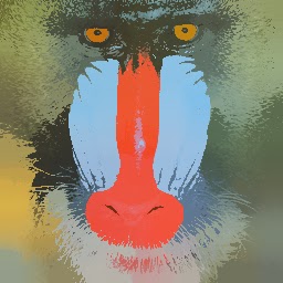
It should be noticed that an image has not only color information but also location one. Since the smoothing procedure explained above ignores location information, two distantly-positioned objects that happen to have similar color can be labeled by the same color. When we would like to assign the different labels to them, we cannot employ the procedure. D. Comaniciu and P. Meer expanded the vector $(r,g,b)$ that represents each pixel to the 5-dimensional vector $(x,y,r,g,b)$ which includes location information $(x,y)$1,2. In this case, the kernel used in the Mean Shift analysis is modified as \begin{equation} K(\vec{x}_i;\;\vec{x},h)=K_{\rm spatial}(\vec{x}_i^{\;s};\;\vec{x}^{\;s},h_s)\;K_{\rm range}(\vec{x}_i^{\;r};\;\vec{x}^{\;r},h_r) \end{equation} where $\vec{x}=(\vec{x}^{\;s},\vec{x}^{\;r})$, $\vec{x}^{\;s}=(x,y)$, $\vec{x}^{\;r}=(r,g,b)$, $h_s$ is the radius of the sphere in the spatial space , and $h_r$ is the the radius of the sphere in the color space. Using the kernel, the mean is calculated by the following expression: \begin{equation} \vec{m}(\vec{x}) = \frac{\sum_{i=1}^{n}\;K(\vec{x}_i;\;\vec{x},h)\;\vec{x}_i}{\sum_{i=1}^{n}\;K(\vec{x}_i;\;\vec{x},h)}. \end{equation} Only when calculating the kernel, $\vec{x}^{\;s}$ and $\vec{x}^{\;r}$ are distinguished. Other calculation is the same as the previous page. Applying the Mean Shift analysis to all points $\{\vec{x}_{i}|i=1,\cdots,n\}$ in the image, we obtain a set of convergence points $\{\vec{z}_{i}|i=1,\cdots,n\}$. By replacing $\vec{x}_i^{\;r}$ (the color component of the original point) by $\vec{z}_i^{\;r}$ (the color component of the convergence point), we generate a new point $\vec{y}_i=(\vec{x}_i^{\;s},\vec{z}_i^{\;r})$. The image constructed from the set $\{\vec{y}_{i}|i=1,\cdots,n\}$ is the final result.
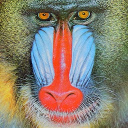
Source Image:
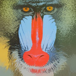
 $(h_s,h_r)=(16,32)$:
 $(h_s,h_r)=(16,64)$:
 The size of the input image is (256,256) pixels. We set
Introduction
In the previous page, I provided a brief explanation of the Mean Shift analysis. In this page, I describe the Mean Shift filtering proposed by D. Comaniciu and P. Meer in [1][2]. I also show the practice of the filtering by the OpenCV library.Theory
Suppose we have an $RGB$ image that consists of $n$ pixels each of which has three values $(r,g,b)$. Since the image is regarded as the distribution of the points in the 3-dimensional space, we can define a density function as shown in the previous discussion. We can detect local maximal points of the density by the Mean Shift analysis as illustrated below. In the figure, the blue circles indicate local maximal points.
It should be noticed that an image has not only color information but also location one. Since the smoothing procedure explained above ignores location information, two distantly-positioned objects that happen to have similar color can be labeled by the same color. When we would like to assign the different labels to them, we cannot employ the procedure. D. Comaniciu and P. Meer expanded the vector $(r,g,b)$ that represents each pixel to the 5-dimensional vector $(x,y,r,g,b)$ which includes location information $(x,y)$1,2. In this case, the kernel used in the Mean Shift analysis is modified as \begin{equation} K(\vec{x}_i;\;\vec{x},h)=K_{\rm spatial}(\vec{x}_i^{\;s};\;\vec{x}^{\;s},h_s)\;K_{\rm range}(\vec{x}_i^{\;r};\;\vec{x}^{\;r},h_r) \end{equation} where $\vec{x}=(\vec{x}^{\;s},\vec{x}^{\;r})$, $\vec{x}^{\;s}=(x,y)$, $\vec{x}^{\;r}=(r,g,b)$, $h_s$ is the radius of the sphere in the spatial space , and $h_r$ is the the radius of the sphere in the color space. Using the kernel, the mean is calculated by the following expression: \begin{equation} \vec{m}(\vec{x}) = \frac{\sum_{i=1}^{n}\;K(\vec{x}_i;\;\vec{x},h)\;\vec{x}_i}{\sum_{i=1}^{n}\;K(\vec{x}_i;\;\vec{x},h)}. \end{equation} Only when calculating the kernel, $\vec{x}^{\;s}$ and $\vec{x}^{\;r}$ are distinguished. Other calculation is the same as the previous page. Applying the Mean Shift analysis to all points $\{\vec{x}_{i}|i=1,\cdots,n\}$ in the image, we obtain a set of convergence points $\{\vec{z}_{i}|i=1,\cdots,n\}$. By replacing $\vec{x}_i^{\;r}$ (the color component of the original point) by $\vec{z}_i^{\;r}$ (the color component of the convergence point), we generate a new point $\vec{y}_i=(\vec{x}_i^{\;s},\vec{z}_i^{\;r})$. The image constructed from the set $\{\vec{y}_{i}|i=1,\cdots,n\}$ is the final result.
Practice by OpenCV
We can usecv::pyrMeanShiftFiltering. The sample code is as follows:
The function cv::pyrMeanShiftFiltering is called in the 14th line. The first argument is an input image, and the second is an output image. The third and fourth arguments are $h_{s}$ and $h_{r}$, respectively. The sixth argument is the termination criteria for the algorithm. If we use pyramid images in the internal calculation, we have to set the level number of them to the fifth argument. Because this time we apply the Mean Shift analysis to the source image only once, we set it to 0. The resultant images are as follows:
Source Image:
params.max_iteration_count_=30 and params.epsilon_=0.01. Maybe cv::pyrMeanShiftFiltering employs the Fukunaga kernel.
References
- Mean Shift Analysis and Applications, D. Comaniciu and P. Meer, 1999 (pdf)
- Mean Shift: A Robust Approach Toward Feature Space Analysis, D. Comaniciu and P. Meer, 2002 (pdf)
- コンピュータビジョン2 最先端ガイド 第2章, アドコム・メディア株式会社 (in Japanese)
2013年5月19日日曜日
Mean Shift Analysis
in Japanese
 Let us consider a sphere (hypersphere) centered on an arbitrary point $\vec{x}$ with a radius $h$. The centroid $\vec{x}_{\rm c}$ of the points within the sphere gives $f(\vec{x}_{\rm c}) > f(\vec{x})$.
 Replacing $\vec{x}_{c}$ by $\vec{x}$ and repeating the same calculation, the initial point converges to a local maximal point of the density $f(\vec{x})$. The convergence is mathematically proved in [1][2].
The approach for detecting local maximal points on the density function $f(\vec{x})$ by repeating movement to the centroid (mean) is referred to as the Mean Shift analysis.
Replacing $\vec{x}_{c}$ by $\vec{x}$ and repeating the same calculation, the initial point converges to a local maximal point of the density $f(\vec{x})$. The convergence is mathematically proved in [1][2].
The approach for detecting local maximal points on the density function $f(\vec{x})$ by repeating movement to the centroid (mean) is referred to as the Mean Shift analysis.
The mean $\vec{m}(\vec{x})$ of points within the sphere centered on the point $\vec{x}$ is defined as \begin{equation} \vec{m}(\vec{x}) = \frac{1}{|S_{h}(\vec{x})|}\sum_{\vec{x}_i \in S_{h}(\vec{x})}\;\vec{x}_{i} \end{equation} where $S_{h}(\vec{x})$ indicates a set of points within the sphere centered on $\vec{x}$ with the radius $h$, and $|S_{h}(\vec{x})|$ is the number of points in $S_{h}(\vec{x})$. In order to generalize the discussion, we rewrite the above expression as \begin{equation} \vec{m}(\vec{x}) = \frac{\sum_{i=1}^{n}\;K(\vec{x}_i;\;\vec{x},h)\;\vec{x}_i}{\sum_{i=1}^{n}\;K(\vec{x}_i;\;\vec{x},h)} \end{equation} where the sum is taken over all points we are now considering. The function $K(\vec{x}_i;\;\vec{x},h)$ is defined as \begin{eqnarray} K(\vec{x}_i;\;\vec{x},h)=\left\{ \begin{array}{} 1\;\; {\rm if}\;\;\|\vec{x}-\vec{x}_i\|\leq h\\ 0\;\; {\rm if}\;\;\|\vec{x}-\vec{x}_i\|\gt h \end{array} \right. \label{kernel} \end{eqnarray} . Then, the density function $f(\vec{x})$ is defined by using $K(\vec{x}_i;\;\vec{x},h)$ as \begin{equation} f(\vec{x})=\frac{1}{n\;V_{d}}\;\sum_{i=1}^{n}\;K(\vec{x}_i;\;\vec{x},h) \end{equation} where $V_{d}$ denotes a volume of the $d$-dimensional hypersphere with the radius $h$. Therefore, the following expression is satisfied: \begin{equation} \int\;d\vec{x}\;f(\vec{x}) = 1. \end{equation} The function $K(\vec{x}_i;\;\vec{x},h)$ is called the kernel. The kernel can be extended to various forms other than (\ref{kernel}).
Let us consider a spherically-symmetrical kernel as \begin{equation} K(\vec{x}_i;\;\vec{x},h) = k\left(\left\|\frac{\vec{x}-\vec{x}_i}{h} \right\|^2\right) \end{equation} where $k(x)$ is called the profile. When we write the density function constructed from the the profile as $f_{K}(\vec{x})$, the derivative of it with respect to $\vec{x}$ yields the following equation: \begin{equation} \vec{\nabla}\;f_K(\vec{x})=\frac{2}{n\;V_d\;h^2}\;\sum_{i=1}^{n}\;k^{\prime}\left(\left\|\frac{\vec{x}-\vec{x}_i}{h} \right\|^2\right)\;\left(\vec{x}-\vec{x}_i\right) \end{equation} where $k^{\prime}(x)=dk(x)/dx$. Introducing $g(x)=-k^{\prime}(x)$, we obtain \begin{equation} \vec{\nabla}\;f_K(\vec{x})=\frac{2}{h^2}f_G(\vec{x})\;\vec{s}_G(\vec{x}) \label{mean-shift-relation} \end{equation} where \begin{equation} f_G(\vec{x})=\frac{1}{n\;V_{d}}\;\sum_{i=1}^{n}\;G(\vec{x}_i;\;\vec{x},h) \end{equation} \begin{equation} \vec{s}_G(\vec{x})=\vec{m}_G(\vec{x})-\vec{x} \end{equation} \begin{equation} m_G(\vec{x}) = \frac{\sum_{i=1}^{n}\;G(\vec{x}_i;\;\vec{x},h)\;\vec{x}_i}{\sum_{i=1}^{n}\;G(\vec{x}_i;\;\vec{x},h)} \end{equation} \begin{equation} G(\vec{x}_i;\;\vec{x},h) = g\left(\left\|\frac{\vec{x}-\vec{x}_i}{h} \right\|^2\right). \end{equation} The mean shift vector $\vec{s}_G(\vec{x})$ is the vector from $\vec{x}$ to $\vec{m}_G(\vec{x})$. The eq.(\ref{mean-shift-relation}) means that the mean shift direction, which is calculated using the kernel $G$, coincides with the direction of the gradient of the density $f_K(\vec{x})$.
If the function $k(x)$ is given as \begin{eqnarray} k(x)=\left\{ \begin{array}{} 1-x\;\; &{\rm if}&\;\;x\leq 1\\ 0\;\; &{\rm if}&\;\;x \gt 1 \end{array} \right., \label{epanechnikov} \end{eqnarray} we get the function $g(x)$ as \begin{eqnarray} g(x)=\left\{ \begin{array}{} 1\;\; &{\rm if}&\;\;x\leq 1\\ 0\;\; &{\rm if}&\;\;x \gt 1 \end{array} \right.. \label{fukunaga} \end{eqnarray} That is, the kernel $G(\vec{x}_i;\;\vec{x},h)$ constructed from the profile $g(x)$ equals to the eq.(\ref{kernel}). The kernel $K(\vec{x}_i;\;\vec{x},h)$ constructed from the eq.(\ref{epanechnikov}) is called the Epanechnikov kernel, and the kernel $G(\vec{x}_i;\;\vec{x},h)$ constructed from the eq.(\ref{fukunaga}) is called the Fukunaga kernel. The mean shift direction by the Fukunaga kernel equals to the direction of the gradient of the density defined by the Epanechnikov kernel.
Introduction
In this page, I describe a brief explanation on the Mean Shift analysis1,2. In the next page, I explain the practice by the OpenCV library.Theory
Suppose we have points $\{\vec{x}_{i}|i=1,\cdots,n\}$ in the $d$-dimensional space. We can consider a density function $f(\vec{x})$ that the distribution of them yields. The density has a large value in the area where there are a lot of points, and has a small one in the area where points sparsely exist.

The mean $\vec{m}(\vec{x})$ of points within the sphere centered on the point $\vec{x}$ is defined as \begin{equation} \vec{m}(\vec{x}) = \frac{1}{|S_{h}(\vec{x})|}\sum_{\vec{x}_i \in S_{h}(\vec{x})}\;\vec{x}_{i} \end{equation} where $S_{h}(\vec{x})$ indicates a set of points within the sphere centered on $\vec{x}$ with the radius $h$, and $|S_{h}(\vec{x})|$ is the number of points in $S_{h}(\vec{x})$. In order to generalize the discussion, we rewrite the above expression as \begin{equation} \vec{m}(\vec{x}) = \frac{\sum_{i=1}^{n}\;K(\vec{x}_i;\;\vec{x},h)\;\vec{x}_i}{\sum_{i=1}^{n}\;K(\vec{x}_i;\;\vec{x},h)} \end{equation} where the sum is taken over all points we are now considering. The function $K(\vec{x}_i;\;\vec{x},h)$ is defined as \begin{eqnarray} K(\vec{x}_i;\;\vec{x},h)=\left\{ \begin{array}{} 1\;\; {\rm if}\;\;\|\vec{x}-\vec{x}_i\|\leq h\\ 0\;\; {\rm if}\;\;\|\vec{x}-\vec{x}_i\|\gt h \end{array} \right. \label{kernel} \end{eqnarray} . Then, the density function $f(\vec{x})$ is defined by using $K(\vec{x}_i;\;\vec{x},h)$ as \begin{equation} f(\vec{x})=\frac{1}{n\;V_{d}}\;\sum_{i=1}^{n}\;K(\vec{x}_i;\;\vec{x},h) \end{equation} where $V_{d}$ denotes a volume of the $d$-dimensional hypersphere with the radius $h$. Therefore, the following expression is satisfied: \begin{equation} \int\;d\vec{x}\;f(\vec{x}) = 1. \end{equation} The function $K(\vec{x}_i;\;\vec{x},h)$ is called the kernel. The kernel can be extended to various forms other than (\ref{kernel}).
Let us consider a spherically-symmetrical kernel as \begin{equation} K(\vec{x}_i;\;\vec{x},h) = k\left(\left\|\frac{\vec{x}-\vec{x}_i}{h} \right\|^2\right) \end{equation} where $k(x)$ is called the profile. When we write the density function constructed from the the profile as $f_{K}(\vec{x})$, the derivative of it with respect to $\vec{x}$ yields the following equation: \begin{equation} \vec{\nabla}\;f_K(\vec{x})=\frac{2}{n\;V_d\;h^2}\;\sum_{i=1}^{n}\;k^{\prime}\left(\left\|\frac{\vec{x}-\vec{x}_i}{h} \right\|^2\right)\;\left(\vec{x}-\vec{x}_i\right) \end{equation} where $k^{\prime}(x)=dk(x)/dx$. Introducing $g(x)=-k^{\prime}(x)$, we obtain \begin{equation} \vec{\nabla}\;f_K(\vec{x})=\frac{2}{h^2}f_G(\vec{x})\;\vec{s}_G(\vec{x}) \label{mean-shift-relation} \end{equation} where \begin{equation} f_G(\vec{x})=\frac{1}{n\;V_{d}}\;\sum_{i=1}^{n}\;G(\vec{x}_i;\;\vec{x},h) \end{equation} \begin{equation} \vec{s}_G(\vec{x})=\vec{m}_G(\vec{x})-\vec{x} \end{equation} \begin{equation} m_G(\vec{x}) = \frac{\sum_{i=1}^{n}\;G(\vec{x}_i;\;\vec{x},h)\;\vec{x}_i}{\sum_{i=1}^{n}\;G(\vec{x}_i;\;\vec{x},h)} \end{equation} \begin{equation} G(\vec{x}_i;\;\vec{x},h) = g\left(\left\|\frac{\vec{x}-\vec{x}_i}{h} \right\|^2\right). \end{equation} The mean shift vector $\vec{s}_G(\vec{x})$ is the vector from $\vec{x}$ to $\vec{m}_G(\vec{x})$. The eq.(\ref{mean-shift-relation}) means that the mean shift direction, which is calculated using the kernel $G$, coincides with the direction of the gradient of the density $f_K(\vec{x})$.
If the function $k(x)$ is given as \begin{eqnarray} k(x)=\left\{ \begin{array}{} 1-x\;\; &{\rm if}&\;\;x\leq 1\\ 0\;\; &{\rm if}&\;\;x \gt 1 \end{array} \right., \label{epanechnikov} \end{eqnarray} we get the function $g(x)$ as \begin{eqnarray} g(x)=\left\{ \begin{array}{} 1\;\; &{\rm if}&\;\;x\leq 1\\ 0\;\; &{\rm if}&\;\;x \gt 1 \end{array} \right.. \label{fukunaga} \end{eqnarray} That is, the kernel $G(\vec{x}_i;\;\vec{x},h)$ constructed from the profile $g(x)$ equals to the eq.(\ref{kernel}). The kernel $K(\vec{x}_i;\;\vec{x},h)$ constructed from the eq.(\ref{epanechnikov}) is called the Epanechnikov kernel, and the kernel $G(\vec{x}_i;\;\vec{x},h)$ constructed from the eq.(\ref{fukunaga}) is called the Fukunaga kernel. The mean shift direction by the Fukunaga kernel equals to the direction of the gradient of the density defined by the Epanechnikov kernel.
References
- Mean Shift Analysis and Applications, D. Comaniciu and P. Meer, 1999 (pdf)
- Mean Shift: A Robust Approach Toward Feature Space Analysis, D. Comaniciu and P. Meer, 2002 (pdf)
- コンピュータビジョン2 最先端ガイド 第2章, アドコム・メディア株式会社 (in Japanese)
2013年5月13日月曜日
Mean Shift Filteringの理論と実践
in English
$RGB$ 空間内の任意の3次元ベクトル $\vec{x}$ は、図に見るように、その近傍にある極大値に向かって収束していく。画像内の全ベクトル(全画素)を、それらが収束する極大値の色に置き換えれば、色の平滑化を行うことができる(平滑化後の密度分布関数を緑の線で示した)。
画像は色だけでなく位置の情報も含む。上記の方法は位置を無視しているので、離れた場所にあるオブジェクト $A$ と $B$ が、たまたま類似色であったため、同じ色(同じラベル)に収束してしまうことがある。オブジェクト $A$ と $B$ に異なるラベルを割り振りたい場合、これでは都合が悪い。そこで、D. Comaniciu と P. Meer は、各画素を表現するベクトルを $(r,g,b)$ ではなく位置情報を含む5次元ベクトル $(x,y,r,g,b)$ に拡張することを考えた1,2。このとき、Mean Shiftで使用するカーネルは以下のように変更される。 \begin{equation} K(\vec{x}_i;\;\vec{x},h)=K_{\rm spatial}(\vec{x}_i^{\;s};\;\vec{x}^{\;s},h_s)\;K_{\rm range}(\vec{x}_i^{\;r};\;\vec{x}^{\;r},h_r) \end{equation} ここで、$\vec{x}=(\vec{x}^{\;s},\vec{x}^{\;r})$、$\vec{x}^{\;s}=(x,y)$、$\vec{x}^{\;r}=(r,g,b)$、$h_s$ は位置空間内の球の半径、$h_r$ は色空間内の球の半径である。このカーネルを使い、次式で重心を計算する。 \begin{equation} \vec{m}(\vec{x}) = \frac{\sum_{i=1}^{n}\;K(\vec{x}_i;\;\vec{x},h)\;\vec{x}_i}{\sum_{i=1}^{n}\;K(\vec{x}_i;\;\vec{x},h)} \end{equation} $\vec{x}^{\;s}$ と $\vec{x}^{\;r}$ の区別がなされるのはカーネル計算時のみである。あとの計算はこれまでと同じである。Mean Shiftの手順を画像内の全ての点 $\{\vec{x}_{i}|i=1,\cdots,n\}$ に適用すると、収束点の集合 $\{\vec{z}_{i}|i=1,\cdots,n\}$ を得る。元の点の色成分 $\vec{x}_i^{\;r}$ を、収束点の色成分 $\vec{z}_i^{\;r}$ に置き換えることにより、新たな点 $\vec{y}_i=(\vec{x}_i^{\;s},\vec{z}_i^{\;r})$ を作る。集合 $\{\vec{y}_{i}|i=1,\cdots,n\}$ から構成される画像が求める結果である。
元画像:
$(h_s,h_r)=(16,32)$:
$(h_s,h_r)=(16,64)$:
両者とも
はじめに
前回、Mean Shift の理論をまとめました。今回は、D. Comaniciu と P. Meer により提案された Mean Shift Filtering についてまとめます。理論
$n$ 個の画素から構成される $RGB$ 画像を考える。各画素は $(r,g,b)$ を持つ。3次元空間内の点の分布を考えれば、前回と同様に密度分布関数を定義することができる。点が疎らに存在する領域の密度は低く、点が密に存在する領域の密度は高い。いま、Mean Shiftを用いて密度分布関数の極大値を検出していくと図のようになるであろう(青丸で極大値を表した)。画像は色だけでなく位置の情報も含む。上記の方法は位置を無視しているので、離れた場所にあるオブジェクト $A$ と $B$ が、たまたま類似色であったため、同じ色(同じラベル)に収束してしまうことがある。オブジェクト $A$ と $B$ に異なるラベルを割り振りたい場合、これでは都合が悪い。そこで、D. Comaniciu と P. Meer は、各画素を表現するベクトルを $(r,g,b)$ ではなく位置情報を含む5次元ベクトル $(x,y,r,g,b)$ に拡張することを考えた1,2。このとき、Mean Shiftで使用するカーネルは以下のように変更される。 \begin{equation} K(\vec{x}_i;\;\vec{x},h)=K_{\rm spatial}(\vec{x}_i^{\;s};\;\vec{x}^{\;s},h_s)\;K_{\rm range}(\vec{x}_i^{\;r};\;\vec{x}^{\;r},h_r) \end{equation} ここで、$\vec{x}=(\vec{x}^{\;s},\vec{x}^{\;r})$、$\vec{x}^{\;s}=(x,y)$、$\vec{x}^{\;r}=(r,g,b)$、$h_s$ は位置空間内の球の半径、$h_r$ は色空間内の球の半径である。このカーネルを使い、次式で重心を計算する。 \begin{equation} \vec{m}(\vec{x}) = \frac{\sum_{i=1}^{n}\;K(\vec{x}_i;\;\vec{x},h)\;\vec{x}_i}{\sum_{i=1}^{n}\;K(\vec{x}_i;\;\vec{x},h)} \end{equation} $\vec{x}^{\;s}$ と $\vec{x}^{\;r}$ の区別がなされるのはカーネル計算時のみである。あとの計算はこれまでと同じである。Mean Shiftの手順を画像内の全ての点 $\{\vec{x}_{i}|i=1,\cdots,n\}$ に適用すると、収束点の集合 $\{\vec{z}_{i}|i=1,\cdots,n\}$ を得る。元の点の色成分 $\vec{x}_i^{\;r}$ を、収束点の色成分 $\vec{z}_i^{\;r}$ に置き換えることにより、新たな点 $\vec{y}_i=(\vec{x}_i^{\;s},\vec{z}_i^{\;r})$ を作る。集合 $\{\vec{y}_{i}|i=1,\cdots,n\}$ から構成される画像が求める結果である。
OpenCVによる実践
cv::pyrMeanShiftFilteringを使えば良い。実装例は以下の通り。
14行目でcv::pyrMeanShiftFilteringを呼び出している。第1引数が入力画像、第2引数が出力画像である。第3引数と第4引数はそれぞれ、$h_{s}$と$h_{r}$に相当する。第6引数はアルゴリズムの停止条件である。ピラミッド画像を利用する場合は第5引数にその階層数を指定する。今回は現画像に一度だけ適用したいので0とした。結果は以下の通りである。元画像:
params.max_iteration_count_=30, params.epsilon_=0.01とした。ソースを見ていないのでcv::pyrMeanShiftFilteringの内部で使われているカーネルの具体的な形は分りません。たぶん福永カーネルかな?
参考文献
登録:
投稿 (Atom)