2013年6月29日土曜日

Windows メモ ~ Dllの作り方 ~


はじめに


Visual StudioにてDllを作成する方法は2つある。
  1. declspec(dllexport)を使う方法
  2. declspec(dllexport)を使わない方法
以下これらについてまとめる。作業環境はVisual Studio 2010 Expressである。

declspec(dllexport)を使う方法

  1. Win32コンソールアプリケーションを選択。
  2. アプリケーションの設定で、「DLL」と「空のプロジェクト」を選択。
  3. mydll.hを作成し、以下を記述する。 マクロはプロパティに記述されているものを使うと便利である。ここではDLLWITHEXPORT_EXPORTSを用いた。
    そうでない場合は、下記の.cppの一番先頭(#include "mydll.h"の前)にそのマクロを#defineすること。 Dllをビルドする場合は__declspec(dllexport)が使われ、ヘッダとして公開される場合は__declspec(dllimport)が使われる。
  4. mydll.cppを作成し、以下を記述する。
  5. ビルドする。DebugあるいはReleaseフォルダ内にプロジェクト名と同じ名前の.lib/.dllファイルが作成される。
  6. できあがったDllを使うため、通常のコンソールアプリを作る。
    main.cppを作り、以下を記述する。 「追加のインクルードディレクトリ」にmydll.hへのパス、「追加のライブラリディレクトリ」にDllWithExport.libへのパスを記述する。「追加の依存ファイル」にDllWithExport.libを記述する。DllWithExport.dllを実行ファイルと同じフォルダにコピーするか、VSの検索パスに登録しておく(たとえば環境変数に、dllを含むフォルダへのパスを記入する)。
  7. 実行する。

declspec(dllexport)を使わない方法

  1. 先と同じようにDll用のプロジェクトを作る。
  2. mydll.hを作成し、以下を記述する。__declspec(dllexport)がないことに注意。
  3. cppと同じフォルダ内にmydll.defを作成し、以下を記述する。 LIBRARYと同じ行にdll名(プロジェクト名と同じ名前のdll)を、EXPORTSの下に一行ずつexportする関数名を書く。これがdllexportの役割を果たす。
  4. プロパティの「モジュール定義ファイル」にmydll.defを記述する。
  5. ビルドする。

C#からの呼び出し

  1. 空のプロジェクトを作る。
  2. DllTest.csファイルを作り以下を記述する。 8,9行目でdllから関数addを取り出し、Addという名前の関数を定義している。 同じ名前のまま使用するなら、EntryPointの記述は必要ない。
  3. 実行すると失敗する。 「DLL 'DllWithExport.dll'の'add'というエントリポイントが見つかりません」
  4. dllを作成する際、以下を記述した。 このとき、C++のコンパイラは関数の名前を装飾する。したがって、dllから明示的に関数を取り出す場合、その装飾された名前を指定しなければならない。これを避けるには、Dllを作るとき名前装飾が起こらないようにすればよい。 以下のようにする。 つまり、Cの規約にしたがって関数名を作成する。
  5. これで実行できる。
  6. C++のdoubleとC#のdoubleは自動的に対応付けられる。明示的に対応付けが必要な場合はMarshallingなる機能を使う。

2013年6月26日水曜日

Computational Geometry 〜 Symbolic Perturbation 〜

in Japanese

Introduction

 In the implementation of computational geometry algorithms, it is important to allow numerical calculation to precisely determine the geometric phase structure which depends on the sign of a function $f$. To make the precise judgement, we should use a multiple-precision integer rather than a floating point number in numerical calculation. If floating-point coordinates are given as an input to the algorithm, they just have to be multiplied by a large number and converted to approximated integers. Even if we employ the multiple-precision integer, however, it is impossible to determine the geometric phase structure when ${\rm sign}(f)=0$. The state is called a degeneracy, which occurs when some coordinate values are coincident with each other. It is the symbolic perturbation method that addresses it. In this page, we would like to describe a brief explanation on the method based on the book.

Degeneracy

 In this explanation, we consider the following determinant: \begin{equation} F(P_i,P_j,P_k) = \left| \begin{array}{ccc} 1 & x_i & y_i \\ 1 & x_j & y_j \\ 1 & x_k & y_k \end{array} \right| \end{equation} where $P_i=(x_i,y_i)$, $P_j=(x_j,y_j)$, and $P_k=(x_k,y_k)$. In the case of a right-hand coordinate system, the determinant is used as follows:

When we follow a path $P_i \rightarrow P_j \rightarrow P_k$,

  1. if $F(P_i,P_j,P_k) > 0$, the path turns left at $P_j$.
  2. if $F(P_i,P_j,P_k) < 0$, the path turns right at $P_j$.

The judgement, for example, is used to implement the 2-dimensional convex hull algorithm as shown here. The degeneracy in the judgement occurs when $F(P_i,P_j,P_k) = 0$. 
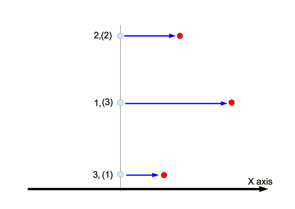
In other words, there exists the point $P_k$ on the line through points $P_i$ and $P_j$ as shown below:

Symbolic Perturbation

 Suppose that the total number of points is $n$. We consider three points of them under the assumption that $i>j>k$. The perturbation is added to each point as follows: \begin{eqnarray} P_i^{\ast}&=&(x_i+\epsilon^{M^i},y_i+\epsilon^{M^{n+i}}) \nonumber \\ &\equiv&(x_i^{\ast},y_i^{\ast}) \end{eqnarray} where $M$ is a large integer and $\epsilon$ is a minutely small quantity. Because we assume $i>j>k$, the sequence of $\{y_i,y_j,y_k,x_i,x_j,x_k\}$ has an ascending order of perturbation amounts. The symbolic perturbation resolves the degeneracies by taking the following steps:
  1. The coordinate value with the largest deviation, that is $x_k$ in the current example, is shifted. Then we trace the path $P_i \rightarrow P_j \rightarrow P_k^{\ast}$.
  2. If we still have the degeneracy, the coordinate value with the second largest deviation, that is $x_j$ in the current example, is shifted. Then we trace the path $P_i \rightarrow P_j^{\ast} \rightarrow P_k^{\ast}$.
  3. The same process is repeated until the degeneracy disappears.
Three degeneracies (a), (b), and (c) in the above figure are resolved as shown below,
where points after perturbations are colored in red, and the path $P_i \rightarrow P_j \rightarrow P_k$ after resolving the degeneracy in blue. The detail procedures to (a), (b), and (c) are as follows:
  1. Only shifting $x_k$, the degeneracy is resolved.
  2. The degeneracy is not resolved by merely shifting $x_k$. The coordinate with the second largest deviation, $x_j$, also must be shifted to resolve the degeneracy.
  3. Since the values, $x_i$, $x_j$, and $x_k$ exist along the $x$ axis, the shifting them does not result in the resolution of the degeneracies. The resolution is achieved only when the coordinate with the next largest deviation, $y_k$, is shifted.
The expansion of $F(P^{\ast}_i,P^{\ast}_j,P^{\ast}_k)$ in power series of $\epsilon$ is as follows: \begin{eqnarray} F(P_i^{\ast},P_j^{\ast},P_k^{\ast}) &=& \left| \begin{array}{ccc} 1 & x_i & y_i \\ 1 & x_j & y_j \\ 1 & x_k & y_k \end{array} \right| \nonumber\\ &&- \left| \begin{array}{ccc} 1 & y_i \\ 1 & y_j \end{array} \right|\;\epsilon^{M^{k}} + \left| \begin{array}{ccc} 1 & y_i \\ 1 & y_k \end{array} \right|\;\epsilon^{M^{j}} - \left| \begin{array}{ccc} 1 & y_j \\ 1 & y_k \end{array} \right|\;\epsilon^{M^{i}}\nonumber\\ &&+ \left| \begin{array}{ccc} 1 & x_i \\ 1 & x_j \end{array} \right|\;\epsilon^{M^{n+k}} - \left| \begin{array}{ccc} 1 & x_i \\ 1 & x_k \end{array} \right|\;\epsilon^{M^{n+j}} + \left| \begin{array}{ccc} 1 & x_j \\ 1 & x_k \end{array} \right|\;\epsilon^{M^{n+i}}\nonumber\\ &&+ \epsilon^{M^{n+k}}(\epsilon^{M^{j}}-\epsilon^{M^{i}}) - \epsilon^{M^{n+j}}(\epsilon^{M^{k}}-\epsilon^{M^{i}}) + \epsilon^{M^{n+i}}(\epsilon^{M^{k}}-\epsilon^{M^{j}}) \label{epsilon_f} \end{eqnarray} The terms in the above expression are arranged in descending order of contributions to $F(P^{\ast}_i,P^{\ast}_j,P^{\ast}_k)$. The processes of resolving degeneracies in (a), (b), and (c) are interpreted by means of the expression as below:
  1. The 1st term in the right-hand side is 0. The 2nd term ($\epsilon^{M^{k}}$'s term) resolves the degeneracy. Since the term has the negative sign, $F(P_i^{\ast},P_j^{\ast},P_k^{\ast})<0$. Therefore, the path turns right at $P_j$.
  2. The 1st and 2nd terms in the right-hand side are 0. The contribution of the 3rd term ($\epsilon^{M^{j}}$'s term) resolves the degeneracy. Since the sign of the term is negative, $F(P_i^{\ast},P_j^{\ast},P_k^{\ast})<0$. Therefore, the path turns right at $P_j$.
  3. The 1st to 4th terms in the right-hand side are all 0. The 5th term ($\epsilon^{M^{n+k}}$'s term) resolves the degeneracy. Since the term has the positive sign, $F(P_i^{\ast},P_j^{\ast},P_k^{\ast})>0$. Therefore, the path turns left at $P_j$.
Moreover, consider the situation that three points overlap as below:
In this case, the 1st to 7th terms in the right-hand side of eq.(\ref{epsilon_f}) are all zero. The 8th term is the contribution of the perturbation to $y_k$. Since $\epsilon^{M^{j}}-\epsilon^{M^{i}}>0$, the sign of the 8th term is positive. Therefore, $F(P_i^{\ast},P_j^{\ast},P_k^{\ast})>0$, so the path turns left at $P_j$.

 From the discussions stated above, the symbolic perturbation method turns out to be the powerful tool to resolve the degeneracies.

Reference

  1. 計算幾何プログラミング, 杉原厚吉, 岩波書店 (written in Japanese)

2013年6月17日月曜日

計算幾何 〜 2次元凸包 理論と実践 〜

in English

はじめに

 前回すこしふれた2次元凸包アルゴリズムについて説明し、C++による実装例を示す。

アルゴリズム

 今回紹介するアルゴリズムは逐次添加法と呼ばれ、$O(n\log{n})$の計算量を持つ1

入力:$A=\{P_1,P_2,\cdots,P_n\}$(添字を固有番号と呼ぶことにする)
出力:凸包 $C(A)$
  1. $A$に属する点を $x$ 座標の小さい順にならべる。この点列を $A^{\prime}=\{P_{(1)},P_{(2)},\cdots,P_{(n)}\}$ と書き、添字を整列番号と呼ぶことにする。$x$ 座標が同じ値を持つ場合は固有番号の大きいものから並べる。整列番号から固有番号へ変換するテーブル $T_{{\rm sorted}\rightarrow{\rm original}}$ を保持しておく。
  2. $A^{\prime}$ の最初の3点から三角形を作り、これを $C(\{P_{(1)},P_{(2)},P_{(3)}\})$ とする。時計回りにたどるときの点列 $V_{\rm clockwise}$ と反時計回りにたどるときの点列 $V_{\rm counterclockwise}$ を保持する。たとえば、時計回りにまわったとき整列番号 $a$ の次に整列番号 $b$ の点がくるなら$V_{\rm clockwise}(a)=b$となるようにすればよい。
  3. 整列番号 $(3)$ から $(n)$ までの点を順に追加する。各点の追加ごとにアルゴリズム $X$(後述)を実行する。
  4. 出力値 $C(\{P_{(1)},P_{(2)},\cdots,P_{(n)}\})$ を得る。$V_{\rm clockwise}$ あるいは $V_{\rm counterclockwise}$ をたどれば、凸包を得ることができる。
 先のページで述べた記号摂動法を適用する際、各座標に以下のように摂動を加える。 \begin{eqnarray} (x_i,y_i)&\rightarrow&(x_i+\epsilon^{M^i},y_i+\epsilon^{M^{n+i}}) \nonumber \\ &\equiv&(x_i^{\ast},y_i^{\ast}) \end{eqnarray} ここで、$n$ は点の総数、$M$ は十分大きな量、$\epsilon$ は十分小さな量である。添字 $i$ として固有番号を採用することにより、たとえ $x$ 座標値が同じであっても、仮想的に $x$ 座標値の小さな順に点を添加していくことができる。たとえば、$x$座標値が同じ3点を考えてみる(下図)。括弧で囲んだ数字は整列番号、囲んでいない番号は固有番号である。$x$ 座標が同じ値を持つ場合は固有番号の大きいものから並べたので、各点の摂動量(青線)と摂動後の点(赤丸)は図のようになる。整列番号の小さい点は摂動量も小さくなることが分る。

 次にアルゴリズム $X$ について述べる。

入力:$C(\{P_{(1)},P_{(2)},\cdots,P_{(k)}\})$、$P_{(k+1)}$、$V_{\rm clockwise}$、$V_{\rm counterclockwise}$、$T_{{\rm sorted}\rightarrow{\rm original}}$
出力:$C(\{P_{(1)},P_{(2)},\cdots,P_{(k+1)}\})$
  1. $P_{(s)}\leftarrow P_{(k)}$
  2. 3点 $P_{(k+1)},P_{(s)},P_{(t)}$ を考える。ここで、$t=V_{\rm counterclockwise}(s)$である。
  3. 3点をこの順にたどったとき右に曲がるなら $s\leftarrow t$ として2へ、左に曲がるなら4へ(下図参照)。
  4. 左に曲がった整列番号$(u)$を保持する。
  5. $P_{(s)}\leftarrow P_{(k)}$
  6. 3点 $P_{(k+1)},P_{(s)},P_{(t)}$ を考える。ここで、$t=V_{\rm clockwise}(s)$である。
  7. 3点をこの順にたどったとき左に曲がるなら $s\leftarrow t$ として6へ、右に曲がるな8へ。
  8. 右に曲がった整列番号$(l)$を保持する。
  9. $V_{\rm counterclockwise}(l)=k+1$、$V_{\rm counterclockwise}(k+1)=u$ とする。
  10. $V_{\rm clockwise}(u)=k+1$、$V_{\rm clockwise}(k+1)=l$ とする。

 右に曲がる、左に曲がるという判定は先のページで取り上げた判定式 $F$ を使えば良い。
  1. $F(P_{(i)},P_{(j)},P_{(k)})$ を考える。
  2. $T_{{\rm sorted}\rightarrow{\rm original}}$ を使って、整列番号を固有番号に変換する。 \begin{eqnarray} a&=&T_{{\rm sorted}\rightarrow{\rm original}}(i) \nonumber \\ b&=&T_{{\rm sorted}\rightarrow{\rm original}}(j) \nonumber \\ c&=&T_{{\rm sorted}\rightarrow{\rm original}}(k) \nonumber \end{eqnarray}
  3. 固有番号のリスト $L=(a,b,c)$ を大きい順に並べ替え、リスト $L^{\prime}=(a^{\prime},b^{\prime},c^{\prime})$ を作成する。並べ替えの際、奇置換なら $p=-1$、偶置換なら $p=1$ とする。
  4. $F(P_{a^{\prime}},P_{b^{\prime}},P_{c^{\prime}})$ の正負を判定する。その結果に$p$の値を乗じたものが $F(P_{a},P_{b},P_{c})$ の符号となる。正なら左に折れ、負なら右に折れる。

C++による実装

ソースはここmain関数は以下の通りである。
  1. 16行目から39行目:乱数による点の生成を行っている。
  2. 43行目:テンプレートクラスConvexHull2dのオブジェクトを作成している。ここではテンプレート引数としてintを指定したが、boost::multiprecision::cpp_intを指定することもできる。
  3. 44行目:アルゴリズムを実行している。
  4. 46行目以降:最初に生成した点と凸包を描画している。
  5. 57行目:凸包を構成する点を取り出している。

デモ

開発環境

  1. Mac OS X 10.8.4
  2. プロセッサ:3.06 GHz Intel Core 2 Duo
  3. メモリ:4GB
  4. Xcode4.6.2 with Apple LLVM 4.2(C++ Language Dialect → C++11, C++ Standard Library → libc++)
  5. boost-1.53.0(Apple LLVM 4.2でコンパイルしたもの。こちら
  6. opencv-2.4.5(Apple LLVM 4.2でコンパイルしたもの。こちら

参考文献

  1. 計算幾何プログラミング, 杉原厚吉, 岩波書店

2013年6月11日火曜日

計算幾何 〜 記号摂動法 〜

in English

はじめに

 計算幾何アルゴリズムの実装において大切なことは、幾何対象の位相構造を数値計算により正しく判定することである。これを実現するため、数値計算には浮動小数点ではなく十分おおきなビット幅を持つ整数(多倍長整数)を使うべきである。たとえば、入力座標値が浮動小数点ならばその座標値に十分大きな数をかけ、その結果を整数に近似すれば良い。しかし、全く同じ座標値を持つ点(縮退あるいは退化と呼ぶ)が作り出す位相構造の判定は依然として困難である。これを解決するのが記号摂動法と呼ばれる手法である。今回はこの手法について参考書籍をもとに議論したい。

退化

 ここでは、2次元凸包を実装する際に必要となる以下の判定式を取り上げる(2次元凸包についてはこちらで解説した)。 \begin{equation} F(P_i,P_j,P_k) = \left| \begin{array}{ccc} 1 & x_i & y_i \\ 1 & x_j & y_j \\ 1 & x_k & y_k \end{array} \right| \end{equation} ここで、$P_i=(x_i,y_i)$、$P_j=(x_j,y_j)$、$P_k=(x_k,y_k)$である。右手系の座標系を考えた場合、上の判定式は次のように使用される。

$P_i \rightarrow P_j \rightarrow P_k$の順にたどったとき、

  1. $F(P_i,P_j,P_k) > 0$ならば$P_j$で左に折れる
  2. $F(P_i,P_j,P_k) < 0$ならば$P_j$で右に折れる

この判定で問題となる退化とは$F(P_i,P_j,P_k) = 0$の場合である。つまり、$P_i$と$P_j$の作る直線の上に$P_k$が存在する場合である(下図)。

記号摂動法

 点の総数を$n$、考察する3点の添字について$i>j>k$が成立しているとする。 $M$を十分大きな整数、$\epsilon$を十分小さい量とし、各点に摂動を加える。 \begin{eqnarray} P_i^{\ast}&=&(x_i+\epsilon^{M^i},y_i+\epsilon^{M^{n+i}}) \nonumber \\ &\equiv&(x_i^{\ast},y_i^{\ast}) \end{eqnarray} $i>j>k$としたから、摂動量は$y_i,y_j,y_k,x_i,x_j,x_k$の順に大きくなる。記号摂動法は以下の手順を踏むことにより退化を解く。
  1. 一番摂動量の大きい座標をずらす。いまの場合、$x_k$である。この状態で$P_i \rightarrow P_j \rightarrow P_k$の順にたどり、判定を行う。
  2. まだ退化していれば、次に摂動量の大きい座標をずらす。いまの場合、$x_j$である。この状態で$P_i \rightarrow P_j \rightarrow P_k$の順にたどり、判定を行う。
  3. 以下同じである。退化が解けるまで続ける。
上の図に摂動を加え、退化を解いたものを以下に示す。摂動を加えた点を赤丸で、退化が解けたときの$P_i \rightarrow P_j \rightarrow P_k$の軌跡を青線で示した。
図の(a)〜(c)に適用される各手順は以下の通りである。
  1. $x_k$をずらす。この時点で退化は解ける。
  2. $x_k$をずらしても退化は解けない。次に摂動量の大きい$x_j$をずらした時点で退化は解ける。
  3. $x$軸に沿って$x_i,x_j,x_k$が存在するから、これらをずらしても退化は解けない。次に摂動量の大きい$y_k$をずらして初めて退化が解ける。
この振る舞いを式で示すため、$F(P^{\ast}_i,P^{\ast}_j,P^{\ast}_k)$を微小量$\epsilon$で展開する。 \begin{eqnarray} F(P_i^{\ast},P_j^{\ast},P_k^{\ast}) &=& \left| \begin{array}{ccc} 1 & x_i & y_i \\ 1 & x_j & y_j \\ 1 & x_k & y_k \end{array} \right| \nonumber\\ &&- \left| \begin{array}{ccc} 1 & y_i \\ 1 & y_j \end{array} \right|\;\epsilon^{M^{k}} + \left| \begin{array}{ccc} 1 & y_i \\ 1 & y_k \end{array} \right|\;\epsilon^{M^{j}} - \left| \begin{array}{ccc} 1 & y_j \\ 1 & y_k \end{array} \right|\;\epsilon^{M^{i}}\nonumber\\ &&+ \left| \begin{array}{ccc} 1 & x_i \\ 1 & x_j \end{array} \right|\;\epsilon^{M^{n+k}} - \left| \begin{array}{ccc} 1 & x_i \\ 1 & x_k \end{array} \right|\;\epsilon^{M^{n+j}} + \left| \begin{array}{ccc} 1 & x_j \\ 1 & x_k \end{array} \right|\;\epsilon^{M^{n+i}}\nonumber\\ &&+ \epsilon^{M^{n+k}}(\epsilon^{M^{j}}-\epsilon^{M^{i}}) - \epsilon^{M^{n+j}}(\epsilon^{M^{k}}-\epsilon^{M^{i}}) + \epsilon^{M^{n+i}}(\epsilon^{M^{k}}-\epsilon^{M^{j}}) \label{epsilon_f} \end{eqnarray} 上式は寄与の大きなものから順に並んでいる。(a)〜(c)において退化が解ける様子をこの式を用いて示すことができる。
  1. 右辺第1項は0である。第2項($\epsilon^{M^{k}}$の項)の寄与により退化が解ける。第2項の符号は負であるから$F(P_i^{\ast},P_j^{\ast},P_k^{\ast})<0$となり、$P_j$で右に折れる。
  2. 右辺は第2項まで0である。第3項($\epsilon^{M^{j}}$の項)の寄与により退化が解ける。第3項の符号は負であるから$F(P_i^{\ast},P_j^{\ast},P_k^{\ast})<0$となり、$P_j$で右に折れる。
  3. 右辺は第4項まで0である。第5項($\epsilon^{M^{n+k}}$の項)の寄与により退化が解ける。第5項の符号は正であるから$F(P_i^{\ast},P_j^{\ast},P_k^{\ast})>0$となり、$P_j$で左に折れる。
さらに、3点が重なった場合を考えてみる。
この場合、式(\ref{epsilon_f})の第7項までは0である。第8項は$y_k$に対する摂動からの寄与である。$\epsilon^{M^{j}}-\epsilon^{M^{i}}>0$であるから第8項の符号は正である。すなわち、$F(P_i^{\ast},P_j^{\ast},P_k^{\ast})>0$となり、$P_j$で左に折れる。
 以上により、記号摂動法を使えば退化を完全に解くことができることがわかる。

参考文献

計算幾何プログラミング, 杉原厚吉, 岩波書店

2013年6月9日日曜日

C++メモ 〜 auto 〜

参照

autoは右辺値の型を表す。ただし、上位のconst&は省かれる。


autoは全てintである。
&は無視されるので、autointである。
ipの型はint*である。autoはそのままint*である。
上位のconst&が無視されるので、autointである。
cipの型は、pointer to const intである。ここに現れるconstは上位のものではない。したがって、autoconst int*である。
ipcの型は、const pointer to intである。ここに現れるconstは上位のものである。したがって、autoint*である。
cipcの型は、const pointer to const intである。上位のconstだけが落とされるので、autoconst int*である。
autostd::initializer_list<int>である。

2013年6月8日土曜日

C++メモ

こう書いたとき何が起きるのか? shared_ptrは強い/弱い参照回数をともに保持する。値渡しが行われると
  1. shared_ptrのcopy contructorが呼ばれる。それに伴い、強い参照回数がincrementされる。引数が一時オブジェクトであれば、 move constructorが呼ばれるので、参照回数は更新されない。しかし、一時オブジェクトが渡されることは稀である。
  2. 関数fから抜ける際、shared_ptrのdestructorが呼ばれる。このとき参照回数が減らされる。
参照回数のincrementとdecrementでは具体的に何が行われるのか?
  1. 参照回数はatomicな共有変数である。したがって、increment/decrementを行うと、共有メモリからの読み出しとそれへの書き込みが同期的に実行される。incrementのばあい適切な最適化が行われるのでそのコストは大きくない。しかし、decrementのときは、処理が複雑なため最適化に制限がかかる。
  2. 同期処理が行われるため、スレッドの数とパフォーマンスの良さが比例しない(scalabilityが失われる)。

こう書いたとき、関数fの引数の寿命について責任を持つのは、呼び出し側である。 すなわち、fは呼び出し側の引数管理の影響を受ける。read-onlyならこう書く。
この場合、引数の所有権は関数fに移り、fのスコープを抜けると同時にそのオブジェクトは破棄される。見方を変えれば、オブジェクトを"吸い込む"関数が必要なら、unique_ptrの値渡しで引数を表現すればよい。上記のconst版は意図が不明瞭である。
前者が意図していることは、関数内部でunique_ptr自身が更新されることである。 一方、後者は意図が不明瞭である。
呼び出し側と呼び出された側で所有権を共有したい場合にこれを使う。
shared_ptr自身を更新したい場合これを使う。
shared_ptr自身を更新する必要があるのかないのか定かでない場合これを使う。

参照

2013年6月1日土曜日

C++メモ

次のFactory関数を考える。 raw pointerを返しているため、だれが所有権を持つのか(だれがdeleteするのか)不明確である。以下のように書くとメモリーリークを起こす。 だれが所有権を持つのかをコメントに残せば良いかもしれない。しかし、最も有効な解決策は、所有権の所在をsignatureとして表現することである。所有権を排他的にしたいなら 共有したいなら となる。これで、こう書いてもメモリーリークはしなくなる。 std::unique_ptrstd::shared_ptrよりオーバヘッドが小さいので を採用すべきである。必要ならいつでもstd::shared_ptrに暗黙変換できる。また、ユーザ定義のスマートポインタへの変換も容易である。 参照