gnuplotの図を保存する。

覚え書き

以下をdecompose_curve.pltとして保存し、 コマンドライン上で を実行すると、指定したディレクトリにこんなpng画像が保存される。

同様に以下をdecompose_surface.pltとして保存し、 以下を実行すると、 こんな画像が保存される。

曲面をグリッドにするには、こんなフォーマットでファイルを作る。 つまり、

1. データを、空行を使って、ブロックに分ける。
2. 各ブロックはX座標あるいはY座標が同じである。

このフォマットを使ったファイル bspline_surface、bezier_surface_0_0、bezier_surface_0_1があるとして、以下のpltファイルを実行すると こうなる。

Coates's Method

in Japanese

1. Introduction

　In recent years a considerable number of studies have been made on the deep learning. The study by A. Coates et al. [1] focused on the reason why the deep learning achieves high performance. I have implemented their algorithm and applied it to the dataset I have at hand. In this page, I will provide a detailed explanation on their algorithm and show my results.

2. Algorithm

　To realize the Coates's method, three datasets are needed:

1. $S_{\rm unsupervised}$ : a dataset to construct the function which maps an image patch to a feature vector
2. $S_{\rm training}$ : a dataset to train the Support Vector Machine (SVM)
3. $S_{\rm test}$ : a dataset to test the SVM

In my study, $S_{\rm unsupervised}$ and $S_{\rm training}$ are the same. First I conduct the following procedures to the dataset $S_{\rm unsupervised}$.

〜 Random Extraction of Patches 〜

1. Extract randomly $n$ patches of $w \times w$ pixels from an image.
2. Arrange pixels in a row from the left-top pixel to the right-bottom one of the patch to make a $N$-dimensional vector $\vec{x}$, where $N=d\times w\times w$ and $d$ is the number of channels. $d=3$ if the patch is color and $d=1$ if it is gray. As in my study the color image is converted to the gray one, $d$ is always 1.
3. If there are $m$ images, the number of $N$-dimensional vectors is $M(=n\times m)$ as $$\begin{equation} \vec{x}^{\;\mu}, \mu=1,\cdots,M \end{equation}$$

〜 Normalization and Whitening 〜

1. For each vector $\vec{x}^{\;\mu}$, the average and the variance are calculated as $$\begin{eqnarray} \bar{x}^{\mu}&=&\frac{1}{N}\sum_{i=1}^{N}x_{i}^{\mu} \nonumber \\ \sigma_{\mu}^2 &=& \frac{1}{N}\sum_{i=1}^{N}\left(x_{i}^{\mu} - \bar{x}^{\mu}\right)^{2}. \nonumber \end{eqnarray}$$ Using them, $\vec{x}^{\;\mu}$ is redefined by $$\begin{equation} x_{i}^{\mu} = \frac{x_{i}^{\mu} - \bar{x}^{\mu} }{ \sqrt{ \sigma_{\mu}^{2}+\epsilon_{\rm n} } }, \end{equation}$$ where $\epsilon_{\rm n}$ is a small value to avoid divide-by-zero. This procedure corresponds to the brightness and contrast normalization of the local area.
2. After normalizing $M$ vectors, they are whitened. Here is the detailed explanation on the whitening.

〜 Clustering 〜

　The $K$-means clustering is applied to $M$ $N$-dimensional vectors. I have fully explained the clustering in this page. $K$ centroids are obtained.

　The image shown below indicates 961 centroids when $K=1000$ and $w=6$. To draw the image, after the elements of each vector are scaled so that they stay within the range of [0,255], the vector is converted to a 6$\times$6 image.

〜 Mapping to Feature Vector 〜

　At this point, the following quantities are obtained:

1. The whitening matrix, $M_{\rm W}$
2. $K$ centroids, $\vec{c}_{\;k}, k=1,\cdots,K$.

Using them, the function which maps a patch to a feature vector is constructed. The procedures are as follows:

1. Arrange pixels in a row from the left-top pixel to the right-bottom one of a path to make a $N$-dimensional vector $\vec{x}$.
2. Normalize the vector $\vec{x}$.
3. Whiten the normalized vector as $\vec{x}_{\rm W} = M_{\rm W}\;\vec{x}$
4. Define the function $f_{k}(\vec{x}_{\rm W})$ as $$\begin{equation} f_{k}(\vec{x}_{\rm W})=\max{\left(0, \mu(z)-z_k\right)}, \nonumber \end{equation}$$ where $$\begin{eqnarray} z_k&=&\|\vec{x}_{\rm W}-\vec{c}_{k} \| \nonumber \\ \mu(z)&=&\frac{1}{K}\sum_{k=1}^{K}z_k. \nonumber \end{eqnarray}$$ $\mu(z)$ is the average distance between the vector $\vec{x}_{\rm W}$ and the $K$ centroids. The function $f_{k}$ outputs 0 if the distance $z_{k}$ between $\vec{x}_{\rm W}$ and the $k$-th centroid $\vec{c}_{k}$ is greater than the average $\mu(z)$ and outputs the finite value $\mu(z) - z_{k}$ if $z_{k}$ is less than $\mu(z)$. In other words in the context of the centroid images shown above, the function $f_{k}$ represents a degree of contribution of $K$ centroids to a patch. The function $f_{k}$ maps a $N$-dimensional vector to a $K$-dimensional vector. This is the feature vector.

Next the following procedures are conducted to the dataset $S_{\rm training}$.

〜 Extraction of Feature Vectors From Training Images〜

1. Suppose that one image is given. The patches of $w\times w$ pixels are sequentially extracted from the image with the step size $s$ (stride).
2. Convert a patch to a $K$-dimensional vector.
3. The entire region which consists of all extracted patches is split into four equal-sized quadrants. Compute the average of the feature vectors in each quadrant. This procedure corresponds to the pooling in the deep learning. It not only decreases the location-dependency but also reduces the dimensionality of the feature vector.
4. The four $K$-dimensional vectors yields a $4K$-dimensional vector. This is the feature vector made from one image. It is used for the classification by the SVM.
5. If there are $D$ images, the number of $4K$-dimensional feature vectors is $D$.
6. Train the SVM by using them.

　In the Coates's method, both the patch extraction and the pooling are executed only once. Moreover, the mapping function $f_{k}$ is computed using the unsupervised learning algorithm ($K$-means clustering). This is why the title of their paper is "Single-Layer Networks in Unsupervised Feature Learning."

Finally, the following procedures are conducted to the dataset $S_{\rm test}$.

〜 Classification of Test Dataset 〜

1. Convert a given image to a $4K$-dimensional feature vector.
2. Classify it by the SVM.

3. Implementation

I have implemented the algorithm in C++ and used the following libraries:

1. opencv2: in order to implement procedures related to the image processing and the $K$-means clustering.
2. boost::numeric::ublas: in order to implement the whitening computation.
3. liblinear: in order to train SVM and classify images.

I have also used the python as a glue that binds procedures together.

4. Image Dataset

　I have used the dataset called LSP15. It can be downloaded by clicking the title "scene category dataset" on this site. It has indoor and outdoor images that are classified into 15 categories. The number of images in each category is about 200 to 300, and image size is approximately 300$\times$300 pixels.
　I have selected two categories and constructed four datasets $S_{\rm training}^{A/B}$ and $S_{\rm test}^{A/B}$.

category	training	test	label
A	1-150 ($S_{\rm training}^{A}$)	151-200 ($S_{\rm test}^{A}$)	-1
B	1-150 ($S_{\rm training}^{B}$)	151-200 ($S_{\rm test}^{B}$)	+1

The name of the image has an integer value like "image_0001.jpg." The integer value in the above table except for labels indicates the image name. The number of the training images and the test images are 150 and 50, respectively. The dataset used for making the feature mapping function $f_{k}$ is $S_{\rm unsupervised}=S_{\rm training}^{A} + S_{\rm training}^{B}$ which contains 300 images. Since the dataset includes 3-channel images (color images), they are converted to the gray images.

5. Parameters

　I have chosen the following parameters:

$n$	$w$	$s$	$K$	$\epsilon_{\rm n}$	$\epsilon_{\rm w}$
50	6	1	1000	10	0.1

$\epsilon_{\rm w}$ is a small value to avoid divide-by-zero in the whitening matrix $M_{\rm W}$ defined by $$\begin{equation} M_{\rm W}=R\;\left(\Lambda+\epsilon_{\rm w}I\right)^{-1/2}\;R^{T}, \label{eq7} \end{equation}$$ where $I$ is the identity matrix. I have already described the detailed explanation on the whitening here.

6. Accuracy

　The results are shown below:

category A	category B	accuracy	accuracy(Hellinger Kernel)
bedroom	CALsuburb	99%(99/100)	97%(97/100)
livingroom	industrial	94%(94/100)	97%(97/100)
MITforest	MITmountain	81%(81/100)	86%(86/100)
industrial	CALsuburb	88%(88/100)	97%(97/100)

　The Hellinger Kernel is able to be introduced by using the linear SVM after computing the square root of the element of the feature vector (Homogeneous Kernel Map).

7. Discussion

1. The accuracies are high in despite of the linear SVM.
2. The Hellinger Kernel is effective except for the pair of bedroom and CALsuburb.
3. The accuracy of the pair of MITforest and MITmountain is low compared with other pairs. If you see the sample images as shown below, it turns out that the images of the two categories are similar.
4. The high performance is achieved without the commonly-used local feature algorithms, e.g. SIFT, SURF, BRIST, and so on. Will the study on them fade out?

　Two test images from each category are shown below:

〜 bedroom 〜

〜 livingroom 〜

〜 MITforest 〜

〜 industrial 〜

〜 MITmountain 〜

〜 CALsuburb 〜

8. References

An Analysis of Single-Layer Networks in Unsupervised Feature Learning, A. Coates, H. Lee, and A. Y. Ng, 2010

Coatesの方法

in English

1. はじめに

　近年、Deep Learning の研究が盛んである。その中にはその高精度の原因を解明しようする研究もある。そのひとつが A.Coates らの "An Analysis of Single-Layer Networks in Unsupervised Feature Learning" である。今回これを実装し手元にある画像に適用してみたのでまとめます。

2. アルゴリズム

　このアルゴリズムを検証するには、3つの画像セットが必要である。

1. 特徴ベクトルを生成する関数を作るための画像セット（$S_{\rm unsupervised}$）
2. 訓練用画像セット（$S_{\rm training}$）
3. テスト用画像セット（$S_{\rm test}$）

今回は、1と2を同じ画像セットとした。以下、アルゴリズムの詳細を順に示す。

最初に、$S_{\rm unsupervised}$ を使用して以下を行う。

〜 パッチの切り出し 〜

1. 1枚の画像からサイズ $w \times w$ のパッチをランダムに $n$ 枚切り出す。
2. 1つのパッチの画素を左上から右下に向かって1列に並べ、$N$ 次元のベクトル $\vec{x}$ を作る。ここで $N=d\times w \times w$、$d$ は画像のチャンネル数である。カラー画像なら3、グレイ画像なら1である。
3. 複数枚の画像について同じことを繰り返す。画像が $m$ 枚あれば $N$ 次元ベクトルは $M(=n\times m)$ 個作られる( $\vec{x}^{\;\mu}, \mu=1,\cdots,M$ )。

〜 正規化と白色化 〜

1. 現在、$M$ 個の$N$ 次元ベクトルがある。個々のベクトルに対し、その成分の平均値と分散を計算し、正規化を行う。 $$\begin{eqnarray} \bar{x}^{\mu}&=&\frac{1}{N}\sum_{i=1}^{N}x_{i}^{\mu} \nonumber \\ \sigma_{\mu}^2 &=& \frac{1}{N}\sum_{i=1}^{N}\left(x_{i}^{\mu} - \bar{x}^{\mu}\right)^{2} \nonumber \end{eqnarray}$$ これらを使って、改めて $\vec{x}^{\;\mu}$ を定義し直す。 $$\begin{equation} x_{i}^{\mu} = \frac{x_{i}^{\mu} - \bar{x}^{\mu} }{ \sqrt{ \sigma_{\mu}^{2}+\epsilon_{\rm n} } } \end{equation}$$ ここで、$\epsilon_{\rm n}$ は0割りを防ぐ微小量である。この作業は、局所領域（パッチ）内での明るさとコントラストの正規化に相当する。
2. 正規化された $M$ 個のベクトルを使って、白色化を行う。白色化の手順はここにまとめてある。

〜 クラスタリング 〜

　$M$ 個の $N$ 次元ベクトルに対し、$K$-meansクラスタリングを行う。クラスタリングの手順はここにまとめてある。$K$ 個の重心が求まる。

　下の画像は $K=1000$ としたときの961個の重心ベクトル（$N=36$次元ベクトル）を画像化したものである（成分の最小値を0に最大値を255に置き換え6$\times$6の画像に変換した）。

〜 特徴ベクトルの作成 〜

　ここまでの手順で以下のものが取得できた。

1. 白色化行列 $M_{\rm W}$
2. $K$ 個の重心座標 $\vec{c}_{\;k}, k=1,\cdots,K$

これらを使って、画像から取り出した1つのパッチから1つの特徴ベクトルを生成する関数を組み立てる。その手順は以下の通りである。

1. パッチの画素を左上から右下に向かって1列に並べ、$N$ 次元のベクトル $\vec{x}$ を作成する。
2. $\vec{x}$ を正規化する。
3. 正規化した $\vec{x}$ に白色化行列 $M_{\rm W}$ をかけて白色化する。$\vec{x}_{\rm W} = M_{\rm W}\;\vec{x}$
4. 関数 $f_{k}(\vec{x}_{\rm W})$ を次式で定義する。 $$\begin{equation} f_{k}(\vec{x}_{\rm W})=\max{\left(0, \mu(z)-z_k\right)} \nonumber \end{equation}$$ ここで、 $$\begin{eqnarray} z_k&=&\|\vec{x}_{\rm W}-\vec{c}_{\;k} \| \nonumber \\ \mu(z)&=&\frac{1}{K}\sum_{k=1}^{K}z_k \nonumber \end{eqnarray}$$ である。つまり、ある点 $\vec{x}_{\rm W}$ に注目したとき、この点と $K$ 個の重心との平均距離を算出する。 そして、平均距離より近い重心のインデックスには有限値を、遠い重心のインデックスには0を割り振る。 上の重心画像を使ってもう少し言い換えると、個々のパッチに対する各重心画像の寄与の度合いを表していることになる。 関数 $f_{k}$ により $N$ 次元ベクトルは、$K$ 次元ベクトルに変換される。これが特徴ベクトルである。

次に、$S_{\rm training}$ に対し以下を行う。

〜 訓練画像からの特徴ベクトルの抽出〜

1. 1枚の訓練画像を考える。サイズ $w\times w$ のパッチを切り出す。その際、次のパッチとの距離（ストライド）を $s$ とする。左上から右下に向かって規則正しくパッチを取り出す。
2. 各パッチから $K$ 次元の特徴ベクトルを算出する。
3. 取り出したパッチが作る全領域を４等分し、各矩形に属する特徴ベクトルの平均ベクトルを計算する。この作業は、Deep LearningにおけるPoolingに相当する。識別対象の位置依存性を減らす手続きでもある。
4. 4つの $K$ 次元ベクトルを並べた4 $K$ 次元ベクトルを、画像1枚に対する特徴ベクトルとする。
5. 全ての訓練画像に対し同じことを繰り返す。訓練画像が $D$ 枚あれば、$D$ 個の4 $K$ 次元ベクトルが作られる。
6. これらを使って、SVMで訓練する。

　上の図を見れば明らかであるが、本手法はパッチの走査とPoolingがそれぞれ一度だけ行われる。また、パッチを特徴ベクトルへ変換する関数 $f_k$ は教師なし学習（$K$-meansクラスタリング）により得られる。よって、Single-Layer Networks in Unsupervised Feature Learning なのである。

最後に、$S_{\rm test}$ に対し以下を行う。

〜 テスト画像の評価 〜

1. 上と全く同じ手順で1枚の画像を4 $K$ 次元の特徴ベクトルに変換する。
2. SVMで識別する。

3. 実装

実装言語はC++、使用したライブラリは以下の通りである。

1. opencv2: 画像周りや $K$-meansクラスタリングなど。
2. boost::numeric::ublas: 白色化の計算など。
3. liblinear: 線形SVMを使った訓練とテスト。

また、アルゴリズムの各手順をつなぎ合わせる際、pythonを使用した。

4. 画像セット

　使用した画像セットはLSP15と呼ばれているものである。ここの scene category dataset という項目をクリックするとダウンロードできる。15個のカテゴリに分類された室内・室外画像である。各カテゴリには、縦横200から300ピクセル程度の画像が200から300枚ほど含まれている。
　今回の検証では、15個のカテゴリから適当に2つを選択し、画像セット $S_{\rm training}^{A/B}$、$S_{\rm test}^{A/B}$ を構成した。

category	training	test	label
A	1-150 ($S_{\rm training}^{A}$)	151-200 ($S_{\rm test}^{A}$)	-1
B	1-150 ($S_{\rm training}^{B}$)	151-200 ($S_{\rm test}^{B}$)	+1

ダウンロードした画像にはimage_0001.jpgのような番号を含む名前が付けられている。上の表の番号はこれを表す。 訓練画像は各カテゴリから150枚、テスト画像は50枚を選択した。 また、関数 $f_{k}$ を作るための画像セット $S_{\rm unsupervised}$は、$S_{\rm training}^{A} + S_{\rm training}^{B}$ とした。総数は300枚である。画像セットにはカラー画像も混ざっているが全てグレー画像に変換して検証を行った。

5. パラメータ

　各種パラメータの値は以下の通りである。

$n$	$w$	$s$	$K$	$\epsilon_{\rm n}$	$\epsilon_{\rm w}$
50	6	1	1000	10	0.1

ここで、$\epsilon_{\rm w}$ は白色化行列 $M_{\rm W}$ の0割りを防ぐ微小量である。 $$\begin{equation} M_{\rm W}=R\;\left(\Lambda+\epsilon_{\rm w}I\right)^{-1/2}\;R^{T} \label{eq7} \end{equation}$$ ただし、$I$ は単位行列である。白色化行列の詳細はここにまとめてある。

6. 識別率

　結果を以下に示す。accuracyは通常の線形SVMを、accuracy(Hellinger Kernel)はHellinger Kernelを使用したときの識別率である。

category A	category B	accuracy	accuracy(Hellinger Kernel)
bedroom	CALsuburb	99%(99/100)	97%(97/100)
livingroom	industrial	94%(94/100)	97%(97/100)
MITforest	MITmountain	81%(81/100)	86%(86/100)
industrial	CALsuburb	88%(88/100)	97%(97/100)

　Hellinger Kernelは、特徴ベクトルの各成分の平方根を計算したあと線形SVMを適用すれば実現できる（Homogeneous Kernel Map）。

7. 考察

1. 線形SVMであるが全般的に識別率は高い。
2. 1つを除いて、Hellinger Kernelの効果は高い。
3. MITforestとMITmountainの組の識別率が他と比べて低いが、下のサンプル画像を見れば納得できると思う。
4. 特別な局所特徴アルゴリズムを使わなくても高い識別率を達成できている。局所特徴アルゴリズムの研究は廃れていくのだろうか？

以下に各カテゴリのテスト画像の例を示す。

〜 bedroom 〜

〜 livingroom 〜

〜 MITforest 〜

〜 industrial 〜

〜 MITmountain 〜

〜 CALsuburb 〜

Boltzmann Machineの基礎

はじめに

Boltzmann Machineについてまとめる。

目的

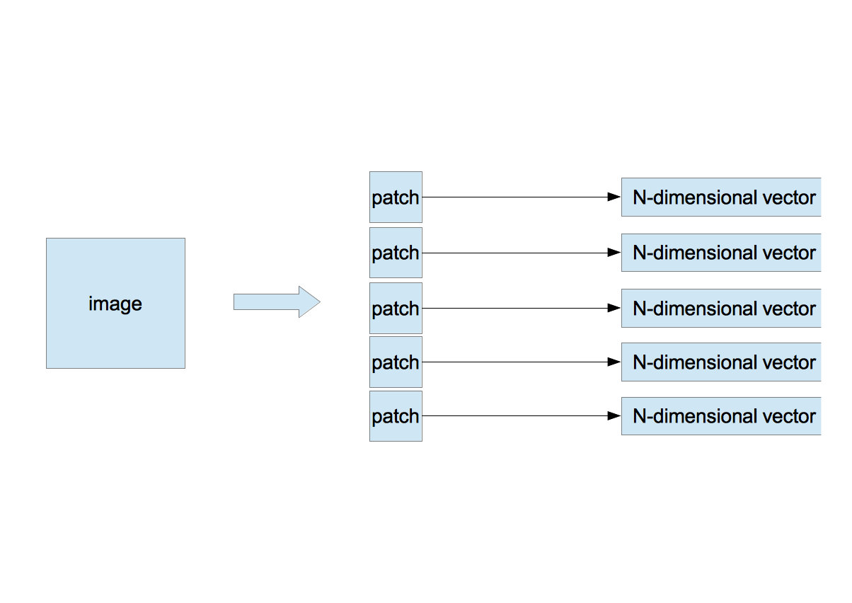
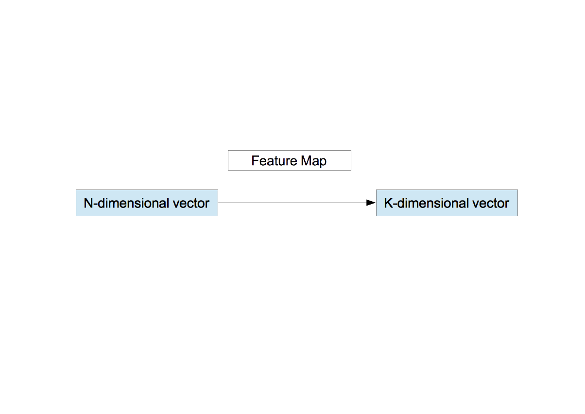
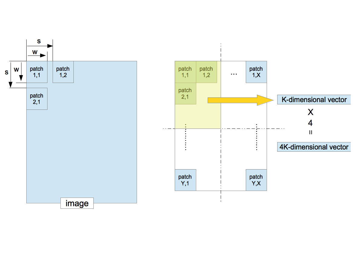
　幅 $w$、高さ $h$ の白黒画像を考える。各画素の値 0 と 255 を -1 と 1 で表し、画像の左上から右下に向かって画素値を並べると、1つの $n$ 次元ベクトル ${\bf x}$ (観測値)となる。ここで、$n=w\times h$ とした。$N$ 枚の画像があれば、$N$ 個の $n$ 次元ベクトル ${\bf x}^{\mu},\;\mu=1,\cdots,N$ を得ることができる。いま、確率分布 $P({\bf X}|\Theta)$ を適当に仮定する。ここで、${\bf X}=\left\{X_{i}\in \left\{-1,1\right\} |\; i=1,\cdots,n \right\}$ は $n$ 次元の確率変数、$\Theta$ は適当なパラメータの集合を表す。観測値 ${\bf x}^{\mu}$ は、確率分布 $P({\bf X}|\Theta)$ に従ってサンプルされた1つの実現値であると解釈する。パラメータ $\Theta$ を調節し、観測値 ${\bf x}^{\mu}$ が従う確率分布 $P({\bf X}|\Theta)$を求めることがここでの目的である。

Boltzmann 分布

　確率分布 として次のBoltzmann 分布を仮定する。 $$\begin{equation} P_{B}({\bf X}|{\boldsymbol \theta}, {\boldsymbol \omega}) = \frac{1}{ Z_{B}({\boldsymbol \theta}, {\boldsymbol \omega}) } \exp\left[-\Phi({\bf X}|{\boldsymbol \theta}, {\boldsymbol \omega})\right] \label{boltzmann} \end{equation}$$ ここで、$Z_{B}({\boldsymbol \theta}, {\boldsymbol \omega})$ は次式で定義される規格化因子（統計物理学に於ける分配関数）である。 $$\begin{equation} Z_{B}({\boldsymbol \theta}, {\boldsymbol \omega})=\sum_{X_1=\pm1}\cdots \sum_{X_n=\pm1}\;\exp\left[-\Phi({\bf X}|{\boldsymbol \theta}, {\boldsymbol \omega})\right] \end{equation}$$ また、$\Phi({\bf X}|{\boldsymbol \theta}, {\boldsymbol \omega})$ はエネルギー関数と呼ばれ、次式で定義される。 $$\begin{equation} \Phi({\bf X}|{\boldsymbol \theta}, {\boldsymbol \omega}) = -\sum_{i\in \Omega}\;\theta_{i}\;X_{i} - \sum_{(i,j)\in E} \omega_{ij}\;X_{i}\;X_{j} \end{equation}$$ $\Omega$ は全画素の集合、$E$ は隣接画素の集合である。エネルギー関数は2つのことを表現している。

1. $\theta_i > 0$ なら、画素値が1である画素が多いほど第1項は小さくなる。$\theta_i < 0$なら、画素値が-1である画素が多いほど第1項は小さくなる。
2. $\omega_{ij} > 0$ なら、画素値の等しい隣接画素が多いほど第2項は小さくなる。$\omega_{ij} < 0$ なら、画素値の異なる隣接画素が多いほど第2項は小さくなる。

第1項をバイアス項、第2項を相互作用項(平滑化項)と呼ぶ。式($\ref{boltzmann}$)の形から、エネルギーが低いほど確率は高くなることが分る。確率分布としてBoltzmann分布を仮定することにより、観測値 ${\bf x}^{\mu}$ の統計性を再現するように2つのパラメータ $({\boldsymbol \theta},{\boldsymbol \omega})$ を求める問題に帰着した。

最尤法

　全観測値 $D=\left\{{\bf x}^{\mu}\;|\;\mu=1,\cdots,N\right\}$ の出現確率は、各観測値の出現確率の積で与えられる。 $$\begin{equation} L_{D}({\boldsymbol \theta},{\boldsymbol \omega})=\prod_{\mu=1}^{N}\;P_{B}({\bf x}^{\mu}|{\boldsymbol \theta}, {\boldsymbol \omega}) \label{ld} \end{equation}$$ ここで、確率変数 ${\bf X}$ ではなく観測値 ${\bf x}^{\mu}$ を使用していることに注意する。$L_{D}$ が最大となるようにパラメータ $({\boldsymbol \theta}, {\boldsymbol \omega})$ を決める手法を最尤法(Maximum Likelihood Estimation)と呼ぶ。実際の計算では、式($\ref{ld}$)の右辺の対数を取った量 $$\begin{equation} L_{D}({\boldsymbol \theta},{\boldsymbol \omega})=\sum_{\mu=1}^{N}\;\ln{P_{B}({\bf x}^{\mu}|{\boldsymbol \theta}, {\boldsymbol \omega})} \label{logld} \end{equation}$$ の最大化を行う。
　$\theta_i$で微分し結果を0とおく。 $$\begin{eqnarray} \frac{\partial L_{D}({\boldsymbol \theta},{\boldsymbol \omega})}{\partial \theta_i}&=& \sum_{\mu}\;\frac{1}{P_{B}({\bf x}^{\mu}|{\boldsymbol \theta}, {\boldsymbol \omega})}\; \frac{\partial P_{B}({\bf x}^{\mu}|{\boldsymbol \theta}, {\boldsymbol \omega})}{\partial \theta_i}\nonumber\\ &=&0 \label{eq10} \end{eqnarray}$$ いま、 $$\begin{eqnarray} \frac{\partial P_{B}({\bf x}^{\mu})}{\partial \theta_i}&=& -\frac{1}{Z_{B}^2}\; \frac{\partial Z_{B}}{\partial \theta_i}\;\exp\left[-\Phi({\bf x}^{\mu})\right] -\frac{1}{Z_B}\;\exp\left[-\Phi({\bf x}^{\mu})\right] \frac{\partial \Phi({\bf x}^{\mu})}{\partial \theta_i}\label{eq11} \\ \frac{\partial \Phi({\bf x}^{\mu})}{\partial \theta_i} &=&-x^{\mu}_i \label{eq12} \\ \frac{\partial Z_{B}}{\partial \theta_i} &=& \sum_{X_1=\pm1}\cdots \sum_{X_n=\pm1}\;X_i\exp\left[-\Phi({\bf X})\right] \label{eq13} \end{eqnarray}$$ が成り立ち(余白の都合上、$({\boldsymbol \theta}, {\boldsymbol \omega})$を省略した)、式($\ref{eq12}$)($\ref{eq13}$)を式($\ref{eq11}$)に代入すると $$\begin{eqnarray} \frac{\partial P_{B}({\bf x}^{\mu})}{\partial \theta_i}&=& -\frac{1}{Z_{B}^2}\; \left\{ \sum_{X_1=\pm1}\cdots \sum_{X_n=\pm1}\;X_i\exp\left[-\Phi({\bf X})\right] \right\} \exp\left[-\Phi({\bf x}^{\mu})\right] \nonumber \\ &&\hspace{1cm}+\frac{1}{Z_B}\;\exp\left[-\Phi({\bf x}^{\mu})\right] x^{\mu}_i \nonumber \\ &=& -\frac{P_{B}({\bf x}^{\mu})}{Z_{B}}\; \left\{ \sum_{X_1=\pm1}\cdots \sum_{X_n=\pm1}\;X_i\exp\left[-\Phi({\bf X})\right] \right\} +P_{B}({\bf x}^{\mu})\; x^{\mu}_i \label{eq14} \end{eqnarray}$$ を得る。式($\ref{eq14}$)を式($\ref{eq10}$)に代入して $$\begin{equation} \sum_{\mu}\; \frac{1}{Z_{B}}\; \left\{ \sum_{X_1=\pm1}\cdots \sum_{X_n=\pm1}\;X_i\exp\left[-\Phi({\bf X})\right] \right\} =\sum_{\mu}\; x^{\mu}_i \end{equation}$$ を得る。左辺の$\mu$についての和は$N$に置き換えることができるから $$\begin{equation} \frac{1}{Z_{B}}\; \left\{ \sum_{X_1=\pm1}\cdots \sum_{X_n=\pm1}\;X_i\exp\left[-\Phi({\bf X})\right] \right\} =\frac{1}{N}\sum_{\mu}\; x^{\mu}_i \label{eq15} \end{equation}$$ が成り立つ。 確率変数についての期待値を $$\begin{equation} E_B(v) = \frac{1}{Z_{B}}\; \left\{ \sum_{X_1=\pm1}\cdots \sum_{X_n=\pm1}\;v\;\exp\left[-\Phi({\bf X})\right] \right\} \end{equation}$$ と表記すれば式($\ref{eq15}$)は $$\begin{equation} E_B(X_i) =\frac{1}{N}\sum_{\mu}\; x^{\mu}_i \label{boltzmann1} \end{equation}$$ と書くことができる。ここで、観測値に対する経験分布を定義する。 $$\begin{equation} Q_{D}({\bf X}) = \frac{1}{N}\;\sum_{\mu}\;\delta({\bf X},\vec{x}^{\;\mu}) \label{empirical} \end{equation}$$ すなわち、変数 ${\bf X}$ が観測値 $\vec{x}^{\;\mu}$ と一致した場合に $1/N$ を、それ以外の場合は0を返す関数である。 これを使うと式($\ref{boltzmann1}$)は $$\begin{equation} E_B(X_i) =\sum_{{\bf X}}\; Q_{D}({\bf X})\;X_i \label{boltzmann1-1} \end{equation}$$ と書き換えることができる。 左辺は確率変数についての1次の期待値、右辺は観測値についての1次の期待値である。
　次に、$\omega_{ij}$で微分し結果を0とおく。 $$\begin{eqnarray} \frac{\partial L_{D}({\boldsymbol \theta},{\boldsymbol \omega})}{\partial \omega_{ij}}&=& \sum_{\mu}\;\frac{1}{P_{B}({\bf x}^{\mu}|{\boldsymbol \theta}, {\boldsymbol \omega})}\; \frac{\partial P_{B}({\bf x}^{\mu}|{\boldsymbol \theta}, {\boldsymbol \omega})}{\partial \omega_{ij}}\nonumber\\ &=&0 \label{eq16} \end{eqnarray}$$ さらに、 $$\begin{eqnarray} \frac{\partial P_{B}({\bf x}^{\mu})}{\partial \omega_{ij}}&=& -\frac{1}{Z_{B}^2}\; \frac{\partial Z_{B}}{\partial \omega_{ij}}\;\exp\left[-\Phi({\bf x}^{\mu})\right] -\frac{1}{Z_B}\;\exp\left[-\Phi({\bf x}^{\mu})\right] \frac{\partial \Phi({\bf x}^{\mu})}{\partial \omega_{ij}}\label{eq17} \\ \frac{\partial \Phi({\bf x}^{\mu})}{\partial \omega_{ij}} &=&-x^{\mu}_i x^{\mu}_j \label{eq18} \\ \frac{\partial Z_{B}}{\partial \omega_{ij}} &=& \sum_{X_1=\pm1}\cdots \sum_{X_n=\pm1}\;X_i X_j\exp\left[-\Phi({\bf X})\right] \label{eq19} \end{eqnarray}$$ が成り立つから、同様な計算を繰り返せば、 $$\begin{equation} E_B(X_i X_j) =\sum_{{\bf X}}\; Q_{D}({\bf X})\;X_i X_j \label{boltzmann2} \end{equation}$$ を得る。左辺は確率変数についての2次の期待値、右辺は観測値についての2次の期待値である。式($\ref{boltzmann1-1}$)と($\ref{boltzmann2}$)をBoltzmannの学習方程式と呼ぶ。

計算量の爆発

　これまでの議論から、確率分布 $P_{B}({\bf X}|{\boldsymbol \theta}, {\boldsymbol \omega})$ を決めるには、次のBoltzmannの学習方程式を解けば良いことが分った。 $$\begin{eqnarray} E_B(X_i|{\boldsymbol \theta}, {\boldsymbol \omega}) &=&\frac{1}{N}\sum_{\mu=1}^{N}\; x^{\mu}_i \\ E_B(X_i X_j|{\boldsymbol \theta}, {\boldsymbol \omega}) &=&\frac{1}{N}\sum_{\mu=1}^{N}\; x^{\mu}_i x^{\mu}_j \end{eqnarray}$$ ただし、 $$\begin{equation} E_B(v|{\boldsymbol \theta}, {\boldsymbol \omega}) = \frac{1}{Z_{B}}\; \left\{ \sum_{X_1=\pm1}\cdots \sum_{X_n=\pm1}\;v\;\exp\left[-\Phi({\bf X|{\boldsymbol \theta}, {\boldsymbol \omega}})\right] \right\} \end{equation}$$ である。 学習方程式の右辺は観測値についての期待値であり計算は容易である。一方、左辺は確率変数の取り得る全ての値についての和であり、$2^n$個の項の和を計算しなければならない。 $n$は通常、1000や10000のオーダとなるので、厳密解を得ることは不可能である。

隠れ変数がある場合

　ここでは、何らかの理由により $n$ 個の画素のうち $m$ 個の画素が観測されない場合を考える。観測される画素値を可視変数、観測されない画素値を隠れ変数と呼び、それぞれ ${\bf V}$、${\bf H}$で表すことにする。すなわち ${\bf X}=({\bf V},{\bf H})$ である。画像中の可視画素の集合を $\Gamma$、隠れ画素の集合を $\Lambda$ とする。このとき、Boltzmann関数($\ref{boltzmann}$)は、 $$\begin{equation} P_{B}({\bf V}, {\bf H}|{\boldsymbol \Theta}) = \frac{1}{ Z_{B}({\boldsymbol \Theta}) } \exp\left[-\Phi({\bf V},{\bf H}|{\boldsymbol \Theta})\right] \label{boltzmann-0} \end{equation}$$ と書くことができる。ただし、${\boldsymbol \Theta}=({\boldsymbol \theta}, {\boldsymbol \omega})$ とした。式変形が容易なように、統計物理学で使われる自由エネルギー $F$ を導入する。 $$\begin{equation} F({\bf V}|{\boldsymbol \Theta})= -\ln{ \left( \sum_{H_1=\pm1}\cdots\sum_{H_m\pm1}\; \exp \left[ -\Phi({\bf V},{\bf H}|{\boldsymbol \Theta}) \right] \right) } \label{free} \end{equation}$$ $P_{B}({\bf V}, {\bf H}|{\boldsymbol \Theta})$ を隠れ変数について周辺化したものは、自由エネルギー $F$ を使って 書くことができる。 $$\begin{eqnarray} P_{V}({\bf V}|{\boldsymbol \Theta}) &\equiv& \sum_{H_1}\cdots\sum_{H_m}\;P_{B}({\bf V}, {\bf H}|{\boldsymbol \Theta}) \label{marginalvv}\\ &=&\frac{1}{Z_B({\boldsymbol \Theta})}\; \exp{ \left[ -F\left({\bf V}|{\boldsymbol \Theta}\right) \right] } \label{marginalv} \end{eqnarray}$$ この式を使って次式を最大化することを考える。 $$\begin{equation} L_{D}({\boldsymbol \Theta})=\sum_{\mu=1}^{N}\;\ln{P_{V}(\vec{v}^{\;\mu}|{\boldsymbol \Theta})} \label{logld-0} \end{equation}$$ ここで、$\vec{v}^{\;\mu}$ は可視変数の観測値である。 議論を一般化するため、パラメータ群 ${\boldsymbol \Theta}$ を代表するパラメータ $\xi$ を考え、これによる偏微分を 考える。 $$\begin{equation} \frac{\partial L_D}{\partial \xi} = 0 \Leftrightarrow E_V\left(\frac{\partial F({\bf V}|{\boldsymbol \Theta})}{\partial \xi} \right) = \frac{1}{N}\;\sum_{\mu}\; \frac{\partial F(\vec{v}^{\;\mu}|{\boldsymbol \Theta})}{\partial \xi} \label{general} \end{equation}$$ ここで、${\bf V}$ についての期待値 $$\begin{equation} E_V(\nu)=\sum_{V_1}\cdots \sum_{V_n}\; \nu\;P_{V}({\bf V}|{\boldsymbol \Theta}) \end{equation}$$ を定義した。式($\ref{general}$)の右辺を考える。 $$\begin{eqnarray} \frac{\partial F(\vec{v}^{\;\mu}|{\boldsymbol \Theta})}{\partial \xi} &=& \sum_{{\bf H}} \left\{ \frac{P_B(\vec{v}^{\;\mu}, {\bf H}|{\boldsymbol \Theta})}{\sum_{{\bf H}^{\prime}}\;P_B(\vec{v}^{\;\mu}, {\bf H}^{\prime}|{\boldsymbol \Theta})} \; \frac{\partial \Phi(\vec{v}^{\;\mu},{\bf H}|{\boldsymbol \Theta})}{\partial \xi} \right\} \nonumber \\ &=& \sum_{{\bf H}} \left\{ P_{H/V}({\bf H}|\vec{v}^{\;\mu}, {\boldsymbol \Theta}) \; \frac{\partial \Phi(\vec{v}^{\;\mu},{\bf H}|{\boldsymbol \Theta})}{\partial \xi} \right\} \end{eqnarray}$$ 最後の式で、ベイズの公式 $$\begin{equation} P_{H/V}({\bf H}|\vec{v}^{\;\mu}, {\boldsymbol \Theta}) = \frac{P_B(\vec{v}^{\;\mu}, {\bf H}|{\boldsymbol \Theta})}{\sum_{{\bf H}^{\prime}}\;P_B(\vec{v}^{\;\mu}, {\bf H}^{\prime}|{\boldsymbol \Theta})} \end{equation}$$ を使用した。さらに変形を続けると $$\begin{eqnarray} \frac{1}{N}\;\sum_{\mu}\; \frac{\partial F(\vec{v}^{\;\mu}|{\boldsymbol \Theta})}{\partial \xi} &=& \frac{1}{N}\;\sum_{\mu}\; \sum_{{\bf H}} \left\{ P_{H/V}({\bf H}|\vec{v}^{\;\mu}, {\boldsymbol \Theta}) \; \frac{\partial \Phi(\vec{v}^{\;\mu},{\bf H}|{\boldsymbol \Theta})}{\partial \xi} \right\} \\ &=& \sum_{{\bf V}} \sum_{{\bf H}} \left\{ P_{H/V}({\bf H}|{\bf V}, {\boldsymbol \Theta}) \; \frac{\partial \Phi({\bf V},{\bf H}|{\boldsymbol \Theta})}{\partial \xi} Q_D({\bf V}) \right\} \end{eqnarray}$$ となる。最後の式で経験分布($\ref{empirical}$)を使用した。次に、式($\ref{general}$)の左辺を考える。 $$\begin{equation} \frac{\partial F({\bf V}|{\boldsymbol \Theta})}{\partial \xi} = \sum_{{\bf H}} \left\{ \frac{P_B({\bf V}, {\bf H}|{\boldsymbol \Theta})}{\sum_{{\bf H}^{\prime}}\;P_B({\bf V}, {\bf H}^{\prime}|{\boldsymbol \Theta})} \; \frac{\partial \Phi({\bf V},{\bf H}|{\boldsymbol \Theta})}{\partial \xi} \right\} \end{equation}$$ したがって、 $$\begin{eqnarray} E_V\left(\frac{\partial F({\bf V}|{\boldsymbol \Theta})}{\partial \xi} \right) &=& \sum_{{\bf V}}\sum_{{\bf H}} P_B({\bf V},{\bf H}|{\boldsymbol \Theta}) \; \frac{\partial \Phi({\bf V},{\bf H}|{\boldsymbol \Theta})}{\partial \xi} \end{eqnarray}$$ を得る。ただし、式($\ref{marginalvv}$)を使った。以上の議論から隠れ変数がある場合の学習方程式は $$\begin{equation} \sum_{{\bf V}}\sum_{{\bf H}} P_B({\bf V},{\bf H}|{\boldsymbol \Theta}) \; \frac{\partial \Phi({\bf V},{\bf H}|{\boldsymbol \Theta})}{\partial \xi} = \sum_{{\bf V}} \sum_{{\bf H}} \left\{ P_{H/V}({\bf H}|{\bf V}, {\boldsymbol \Theta}) \; \frac{\partial \Phi({\bf V},{\bf H}|{\boldsymbol \Theta})}{\partial \xi} Q_D({\bf V}) \right\} \end{equation}$$ となる。　$\xi=(\theta_i, \omega_{ij})$ として、次式を得る。 $$\begin{eqnarray} \sum_{{\bf V}}\sum_{{\bf H}} P_B({\bf V},{\bf H}|{\boldsymbol \Theta}) \; X_i &=& \sum_{{\bf V}} \sum_{{\bf H}} \left\{ P_{H/V}({\bf H}|{\bf V}, {\boldsymbol \Theta}) \; X_i \;Q_D({\bf V}) \right\} \\ \sum_{{\bf V}}\sum_{{\bf H}} P_B({\bf V},{\bf H}|{\boldsymbol \Theta}) \; X_i\;X_j &=& \sum_{{\bf V}} \sum_{{\bf H}} \left\{ P_{H/V}({\bf H}|{\bf V}, {\boldsymbol \Theta}) \; X_i\;X_j \;Q_D({\bf V}) \right\} \end{eqnarray}$$ ただし、 $$\begin{equation} X_{i} = \left\{ \begin{array}{l} V_{i}\;(i \in \Gamma) \\ H_{i}\;(i \in \Lambda) \end{array} \right. \end{equation}$$ である。

隠れ変数の意味

　確率分布 $P_B({\bf V}, {\bf H}|{\boldsymbol \Theta})$ を隠れ変数で周辺化して得られる $P_V({\bf V}|{\boldsymbol \Theta})$ のエネルギー関数は、式($\ref{marginalv}$)の形から自由エネルギー $F$ である。 $$\begin{equation} F({\bf V}|{\boldsymbol \Theta})= -\ln{ \left( \sum_{H_1=\pm1}\cdots\sum_{H_m\pm1}\; \exp \left[ -\Phi({\bf V},{\bf H}|{\boldsymbol \Theta}) \right] \right) } \label{free0} \end{equation}$$ $P_B({\bf V}, {\bf H}|{\boldsymbol \Theta})$ のエネルギー関数 $\Phi$ に比べ複雑さが増していることが分る。この複雑さは、分布関数 $P_V({\bf V}|{\boldsymbol \Theta})$ の表現力を高めている。言い換えると、隠れ変数を導入することにより、学習モデルの表現能力は向上するのである。

参考文献

ディープボルツマンマシン入門 ボルツマンマシン学習の基礎, 安田宗樹, 人工知能学会誌 28巻 3号, 2013年5月.

How to install pcl-1.7.1 into iMac (OS X ver. 10.9.4)

in English

最初、macportsを使ってlibpclのインストールを試みた。 依存ファイルのインストールのあと、libpclのコンパイルに失敗。 いろいろ調べてmacportsを諦める。

ここからソースをダウンロードして、解凍。 依存ライブラリは既にmacportsでインストールされている。 途中でエラー。 pcl-pcl-1.7.1/io/include/pcl/io/ply/ply_parser.hに記述してあるtemplateの定義が原因。clangのバグ。 ここを見てソースを修正する。修正後のソースは以下の通り。
at関数の定義を2つ削除。 さらに、at関数の定義を2つ削除。 削除した4つの定義を移動する。 あらためて 今度は、こんなエラー。 ここを見て以下のように修正する。 再度、 今度はこんなエラー すべてのmoduleをコンパイルすることを諦める。コンパイルできないmoduleは、linemod関係のものだけなので、これらをコンパイル対象から外す。pcl-pcl-1.7.1/tools/CMakeLists.txtの114行目から121行目までをコメントアウト。 あらためて、 できた。ここにあるサンプルは動作した。