Scene Recognition by Chainer

in Japanese

Introduction

　In the previous page, a scene recognition (15-class classification) was performed using Caffe. In this page, the same problem is addressed by fine-tuning a pre-trained Caffe model by means of Chainer.

Computation Environment

　　An instance g2.2xlarge in the Amazon EC2 which mounts the GPU device is used.

Dataset

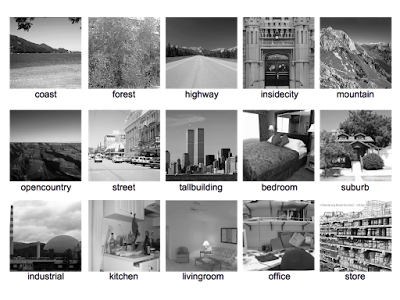
　The CNN is trained on the dataset LSP15 which consists of the 15 directories as follows:

1. MITcoast
2. MITforest
3. MIThighway
4. MITinsidecity
5. MITmountain
6. MITopencountry
7. MITstreet
8. MITtallbuilding
9. bedroom
10. CALsuburb
11. industrial
12. kitchen
13. livingroom
14. PARoffice
15. store

The name of the directory represents the category of the scene. Each directory contains about 200 to 300 images.

Data Augmentation

　In order to augment dataset, the mirror images are added to it. Then the images are divided by the split ratio 6:1. The former group corresponds to a training dataset, and the latter one a testing dataset. The numbers of them are shown below.

label	name	number of train	number of test
0	MITcoast	610	100
1	MIThighway	440	70
2	MITmountain	630	100
3	MITstreet	490	80
4	MITforest	550	90
5	MITinsidecity	520	80
6	MITopencountry	690	110
7	MITtallbuilding	600	100
8	bedroom	360	60
9	CALsuburb	400	60
10	industrial	520	80
11	kitchen	360	60
12	livingroom	490	80
13	PARoffice	360	60
14	store	540	90
		7560	1220

A maximum square centered on an image is resized to $256 \times 256$. Text files in which paths to image files and their labels are described look like this:

--- test.txt ---
--- train_valid.txt ---

Load and Save of Caffe Model

　In this work, bvlc_reference_caffenet.caffemodel that Caffe provides as a pre-trained model is employed. The script to load it is as follows: Since it takes CaffeFunction a long time to load a Caffe model, it is a good idea to save it using cPickle for later reference.

Implementation of Network

　The network equivalent to the Caffe model (bvlc_reference_caffenet.caffemodel) needs to be represented in Chainer before proceeding. The sample code Chainer provides (chainer-1.6.0/examples/imagenet/alex.py) helps us implement it. Referring to the prototxt file distributed with bvlc_reference_caffenet.caffemodel also makes it easy for us to do so. My implementation looks like this:

--- reference_caffenet.py ---
That code makes it easy to implement the class used in the current work. The top layer of the network, fc8, is renamed to scene_fc8, and the number of output units is changed from 1000 to 15. The modified class can be written as follows:

--- modified_reference_caffenet.py ---

Fine-Tuning

　The Caffe model saved using cPickle contains those instances of types L.Convolution2D and L.Linear which have pre-trained parameters $W$s and $b$s. The class ModifiedReferenceCaffeNet defined above has the same layers as the original Caffe model except for the layer scene_fc8. $W$s and $b$s of conv1, conv2, conv3, conv4, conv5, fc6, and fc7 of the original Caffe model are copied to those of the modified model (ModifiedReferenceCaffeNet). Then the modified model is fine-tuned on the current dataset (15-classification dataset).

Training

　The script to train is shown below:

--- train.py ---

1. 15th line : a path to the Caffe model saved using cPickle
2. 16th line ： a path to a file to save the fine-tuned model
3. 17th line ： a path to a mean image path
4. 21st line : a learning rate
5. 22nd line ： a mini batch size
6. 23rd line ： the number of epochs
7. 24th line : a decay rate of the learning rate per epoch
8. 29th line : a path to a training dataset
9. 30th line ： a path to a testing dataset
10. 33〜45th lines : The python function def test calculates both the average loss and the average accuracy over the testing dataset.
11. 52〜63rd lines : These lines load dataset. The class DataLoader is discussed later.
12. 75th line ： The line loads the original Caffe model.
13. 78th line : The line generates an instance of the type ModifiedReferenceCaffeNet.
14. 81st line : The line copies the pre-trained parameters $W$s and $b$s of the original model to those of the instance of the ModifiedReferenceCaffeNet. The top layer scene_fc8 of it has the parameters initialized with default values. The function copy_model is discussed later.
15. 85th line : The line copies the model to the GPU device.
16. 86th line : The line selects the SGD as the optimization algorithm.
17. 87th line : The line passes to the SGD algorithm the model that is to be optimized using the SGD.
18. 93〜115th lines ： These lines are for fine-tuning loop.
19. 123rd line : The line saves the fine-tuned model.

The definitions of DataLoader and ImageCropper are as follows:

--- data_loader.py ---

--- image_cropper.py ---
The function copy_model is described in this page.

Training

　The accuracies and the losses for the training and testing datasets are shown below.

Training dataset

Testing dataset

The accuracy for the testing dataset achieves about 96.23%.

Construction of Classifier

　The class for a classifier is implemented as shown below.

--- modified_reference_caffenet_with_predictor.py ---
The usage of the classifier looks like this:

--- predict.py ---

1. 12th line : a path to the testing dataset
2. 13th line : a path to the mean image
3. 14th line : a path to the fine-tuned model
4. 18th line : The line loads the model.
5. 21st line : The line generates the instance of the class ModifiedReferenceCaffeNetWithPredictor.
6. 24th line : The line copies the parameters to the predictor. If ModifiedReferenceCaffeNetWithPredictor had been used to train the model, this procedure would not have been needed.
7. 27〜32nd lines : The lines load the testing dataset.
8. 35〜40th lines : The lines reduces the number of the testing dataset and construct instances of Variable.
9. 43,44th lines ： The lines classify the data.

The execution of the script predict.py yields the following output. The predictor correctly infers labels except for the first one.

Construction of Feature Extractor

　The following code specifies how feature vectors are extracted from the layer fc7.

--- modified_reference_caffenet_with_feature_extractor.py ---
The following code shows how the data which is passed to liblinear as input argument is generated from the feature vectors.

--- extract.py ---

1. 59th line : The code loads the fine-tuned model.
2. 62nd line : The line generates the extractor.
3. 65th line : The line copies the parameters of the fine-tuned model to those of the extractor
4. 71st line : The line makes input data for liblinear.

Execution of SVM

　The following command is run to train SVM. The following command is run to predict labels. As shown above, the accuracy by Softmax layer achieves 96.23%. The SVM improves it by about 1%.

Fully Convolutional Networks 〜 Chainerによる実装 追記 〜

はじめに

　先のページで Chainer を用いてFully Convolutional Networks（FCN）を簡略化したものを実装した。今回は、同じ問題に対し以下の修正を行った。

1. Batch Normalization 層の導入
2. 訓練データの増量

学習速度は速くなったが、過学習は依然として残ったままである。

Batch Normalization

　原論文はここにある。層間を流れるデータをミニバッチ単位で正規化すると、学習速度が速くなるというものである。幸いなことに Chainer はこれをサポートしているので、以下のように3つの Batch Normalization 層を導入した。

-- myfcn.py -- 49,50,51行目と68,75,82行目が追記したコードである。

データの増量

　訓練データに反転画像を追加し２倍に増やした。

結果

　学習過程の正解率と損失を以下に示す。ここで正解率とは1枚の画像当たり何割の画素が正解したかを全画像について平均したものである。

"no norm"は正規化なし、"no augmentation"はデータ増量なしを表す。上のグラフから分ることは、正規化とデータ増量は伴に学習速度を速くしているということである。 正規化あり、データ増量ありではテスト画像の正解率は0.85程度であり、20Epoch辺りで収束している（ここで言う学習速度とは、どれだけのEpoch数で収束するかを表す。少ないEpoch数で収束するなら学習速度は速いと表現した。データを増量した場合、1Epochの計算に要する時間は倍程度になるので、EC2インスタンスの課金量は変わらない）。しかしながら、テスト画像に於ける損失（期待損失）は依然として途中から上昇してしまう。訓練データが少ないのが原因だろう。

Fully Convolutional Networks 〜 Chainerによる実装 〜

in English

はじめに

　先のページで Chainer を用いてシーン認識を行った。今回は、簡略化した Fully Convolutional Networks（FCN） を Chainer を使って実装してみる。（ここに追記した。)

計算機環境

　これまでと同じく、Amazon EC2 にある g2.2xlarge を利用した。GPU を搭載したインスタンスである。

データセット

　今回使うデータセットは VOC2012 である。以下のような領域分割用の教師データも含まれている。

領域分割の教師データの数は2913枚、これを4:1に分割し、前者を訓練データ、後者をテストデータとした。

number of train	number of test
2330	580

訓練データ数は10で、テストデータ数は5で割り切れるように端数を切り捨てた（それぞれ訓練時のミニバッチサイズである）。文献のアルゴリズムは任意サイズの画像を受け付けるが、ここでの実装では、簡単のため、固定サイズ（224$\times$224）に制限した。これに伴い、入力画像をあらかじめこのサイズに変換した。

画像の中心部分に収まる最大の正方形をリサイズしただけである。VOC2012では、以下の21クラスを扱う。

label	category
0	background
1	aeroplane
2	bicycle
3	bird
4	boat
5	bottle
6	bus
7	car
8	cat
9	chair
10	cow
11	diningtable
12	dog
13	horse
14	motorbike
15	person
16	potted plant
17	sheep
18	sofa
19	train
20	tv/monitor

ネットワークの構造

　ネットワークの構造は以下の通りである。文献では、pool5 の後ろにも層は存在するが、簡単化のため、これらを削除した。

1. name: 層の名前
2. input: 入力featureマップの1辺のサイズ
3. in_channels: 入力featureマップ数
4. out_channels: 出力featureマップ数
5. ksize: カーネルのサイズ
6. stride: ストライドのサイズ
7. pad: paddingのサイズ
8. output: 出力featureマップの1辺のサイズ

pool3、pool4、pool5 の出力に接続する層を以下に示す。これらの層を通ったあとの出力データ名をp3、p4、p5とする。これら3つのデータのfeatureマップの数はクラスの数に等しくなる。

featureマップを拡大する層（Deconvolution層）は以下の通りである。

p4にupsample_pool4が、p5にupsample_pool5が適用され、これら2つのデータとp3とが加算され、最後にupsample_finalで元画像のサイズに拡大される。これで文献の FCN-8s に相当するものが出来上がる。

ネットワークの実装

　上記の構造をそのままChainerで記述する。

-- myfcn.py -- ラベルは0から20までであるが、物体の境界線には-1を配置し、softmax_cross_entropyの計算時に境界の寄与を無視するようにした（Chainerの仕様ではラベルが-1の画素は評価されない）。また、関数calculate_accuracyでも、境界線上の画素を省くようにしてある。3つのデータを加算する関数 add の定義は以下の通りである。

-- add.py --

訓練

　訓練時のスクリプトは以下の通りである。

-- train.py -- -- mini_batch_loader.py --
関数 copy_model はここに掲載されているものを利用した。VGGNet.pyはここからダウンロードした。train.pyでしていることは、

1. オブジェクトmini_batch_loaderを作る。
2. VGGNet.pyで定義されたネットワークのオブジェクトを作る。
3. MyFcn.pyで定義されたネットワークのオブジェクトを作る。
4. VGGNetのパラメータをMyFcnにコピーする。
5. 最適化アルゴリズムとして MomentumSGD を選択する。
6. あとは、通常の訓練過程である。

データを一括読み込みすると、ビデオメモリーが足りなくなるので、要求されるごとに読み込むようにしてある。

結果

　62エポックで計算を打ち切った。学習時の精度と損失は以下の通りである。

-- 訓練画像--

-- テスト画像 --

1枚の画像の中で何%の画素が正解したかを計算し（境界線上の画素は除く）、全画像について平均したものを正解率（accuracy）と定義した。訓練画像に対しては理想的な振る舞いを示すが、テスト画像に対しては損失が途中から上昇し始めている。過学習しているように見える。最終的な正解率は、訓練画像で0.99、テスト画像で0.82程度である。以下に入力画像、予測画像、教師画像の例を示す。数値はこの画像の正解率である。

以下に、その他の画像の予測例を示す。予測画像と教師画像を並べてある。

-- 訓練画像--

-- テスト画像--

背景で精度を稼いでしまうので、満足の行く結果とするには90%以上の精度を実現する必要がある。