前回、pcl-1.7.1をコンパイルしたときは、
いろいろエラーが出ましたが、pcl-1.7.2は何の問題もなくコンパイルできました。
ここからソースをダウンロードして、解凍。
依存ライブラリは既にmacportsでインストールされている。
2014年12月29日月曜日
2014年11月24日月曜日
1次元ロジスティック回帰と確率的勾配降下法
はじめに
ここでは、1次元ロジスティック回帰と、これを解く際に用いられる確率的勾配降下法についてまとめる。
1次元ロジスティック回帰
2分類問題を考える。$N$ 個の観測値 $\vec{x}^{\;i},i=1,\cdots,N$ が与えられ、それぞれ0か1のラベルを持つとする。このとき、観測値が従う確率分布モデル $p(c=0,1\;|\;\vec{x}\;;\;\vec{\omega},b)$ を求めたい。ここで、$\vec{\omega},b$ はモデルを調節するパラメータである。各観測値が他の観測値の影響を受けないと仮定すれば、全ての観測値の確率は 次式で与えられる。 \begin{equation} L(\vec{\omega},b)=\prod_{i=1}^{N}\;p(c^{i}\;|\;\vec{x}^{\;i}\;;\;\vec{\omega},b) \label{likelihood} \end{equation} これが最大となるように $(\vec{\omega},b)$ を調節すればよい。計算を容易にするため次式の最小化を考える。 \begin{equation} L(\vec{\omega},b)=-\sum_{i=1}^{N}\;\ln{p(c^{i}\;|\;\vec{x}^{\;i}\;;\;\vec{\omega},b)} \label{nll} \end{equation} 上式を負の対数尤度(Negative Log Likelihood:NLL)関数と呼ぶ。ところで、観測値のラベル $c$ を0か1に制限したので、確率 $p$ は以下のように書くことができる。 \begin{equation} p(c\;|\;\vec{x}\;;\;\vec{\omega},b)=s(1\;|\;\vec{x}\;;\;\vec{\omega},b)^c\;\left\{1-s(1\;|\;\vec{x}\;;\;\vec{\omega},b)\right\}^{1-c} \end{equation} ここで、$s$ は $c=1$ となる確率である。$s$ と $\vec{x}$ を結びつけるモデルが必要である。1次元ロジスティック回帰では次のモデルを考える。 \begin{eqnarray} s(1\;|\;\vec{x}\;;\;\vec{\omega},b) &=& \sigma\left(f(\vec{x}\;;\;\vec{\omega},b)\right)\nonumber \\ \sigma(a) &=& \frac{1}{1+\exp{(-a)}}\label{sigmoid}\\ f(\vec{x}\;;\;\vec{\omega},b) &=& \vec{\omega}^{\;T}\cdot\vec{x}+b \label{projection} \end{eqnarray} 関数 $\sigma$ はシグモイド関数と呼ばれ、以下のような形をしている。

- $\vec{\Omega}$に適当な初期値を与える。
- 次式で $\vec{\Omega}$ を更新する。 \begin{equation} \vec{\Omega}\leftarrow \vec{\Omega} - \eta \frac{\partial L(\vec{\Omega})}{\partial \vec{\Omega}} \end{equation} ここで $\eta$ は学習率と呼ばれる正の量である。収束速度を調節するパラメータである。
- $L$ の変化量がしきい値以下となるまで上記を繰り返す。あるいは、エラー $E$ \begin{equation} E=\sum_{i=1}^{N}\;\left|c^{i}-s(1\;|\;\vec{X}^{\;i}\;;\;\vec{\Omega})\right| \end{equation} の変化量がしきい値以下となるまで繰り返しても良い。この量は理想的には0になって欲しい量である。
確率的勾配降下法(Stochastic Gradient Descent:SGD)
式(\ref{gradient})を見て分る通り、通常の勾配降下法では $\vec{\Omega}$ の更新ごとに全観測値についての和を取る必要がある。大規模データの場合、これでは大変時間がかかる。そこで、$\vec{\Omega}$ の更新に使うデータをランダムに取り出すことを考える。この手法を確率的勾配降下法と呼ぶ。 手順は以下の通りである。
- データをシャッフルしたあと、複数のグループに分割する。たとえば、1000個のデータを10個のデータのグループに分割する。各グループはミニバッチ(minibatch)と呼ばれる。
- $\vec{\Omega}$に適当な初期値を与える。
- 次式で $\vec{\Omega}$ を更新する。
- $\mbox{for}\;\;\;\;k = 1, \cdots,$ \begin{equation} \vec{\Omega}\leftarrow \vec{\Omega} - \eta \left\{ -\frac{1}{|\Lambda^{k}|} \sum_{i\;\in\;\Lambda^k}\;\vec{X}^{\;i} \left(c^{i}-s(1\;|\;\vec{X}^{\;i}\;;\;\vec{\Omega})\right) \right\} \label{grad} \end{equation}
- 先の勾配法と同じように何らかの量がしきい値以下となるまで上記を繰り返す。
実装
2次元平面に、(5,5)と(0,0)を中心にした2つの正規分布を使って1000個ずつ点を生成し、2分類問題を行なった。ミニバッチのサイズを10、学習率を0.1とした。Theanoを使って実装を行なった。


2014年11月3日月曜日
Restricted Boltzmann Machine
はじめに
以前、Boltzmann Machineの基礎を解説し、その最後に隠れ変数の意味について述べた。今回はRestricted Boltzmann Machineについて解説する。
Restricted Boltzmann Machine
Restricted Boltzmann Machineとは、可視層(入力層)と隠れ層(出力層)の2層から構成されるBoltzmann Machineである。ユニット間の結合は層間にのみ存在し、同一層内には存在しない(下図参照)。これが名前の由来である。

学習方程式
Restricted Boltzmann Machineの学習モデルは先の解説と同様にBoltzmann関数である。 \begin{equation} P_{B}({\bf V}, {\bf H}|{\boldsymbol \Theta}) = \frac{1}{ Z_{B}({\boldsymbol \Theta}) } \exp\left[-\Phi({\bf V},{\bf H}|{\boldsymbol \Theta})\right] \label{boltzmann-1} \end{equation} 式を扱い易くするため、統計物理学で使用される自由エネルギー $F({\boldsymbol V}|{\boldsymbol \Theta})$ \begin{equation} F({\boldsymbol V}|{\boldsymbol \Theta})= -\ln{ \left( \sum_{H_1=\pm1}\cdots\sum_{H_m\pm1}\; \exp \left[ -\Phi({\bf V},{\bf H}|{\boldsymbol \Theta}) \right] \right) } \label{free} \end{equation} を導入する。このとき正規化因子(分配関数)は次式で与えられる。 \begin{equation} Z_{B}({\boldsymbol \Theta})= \sum_{V_1=\pm1}\cdots\sum_{V_n=\pm1}\; \exp \left[ -F({\boldsymbol V}|{\boldsymbol \Theta}) \right] \end{equation} 式(\ref{energy})を式(\ref{free})に代入する。 \begin{eqnarray} F({\boldsymbol V}|{\boldsymbol \Theta}) &=& -\ln{\left( \sum_{H_1}\cdots\sum_{H_m}\; \exp \left[ \sum_{i\;\in\;\Gamma}\; \theta_{i}^V\;V_{i} +\sum_{j\;\in\;\Lambda}\;\theta_{j}^H\;H_{j} +\sum_{i\;\in\;\Gamma}\;\sum_{j\;\in\;\Lambda} \omega_{ij}\;V_{i}\;H_{j} \right] \right) } \nonumber \\ &=& -\ln{\left( \exp \left[ \sum_{i\;\in\;\Gamma}\; \theta_{i}^V\;V_{i} \right] \sum_{H_1=\pm 1}\cdots\sum_{H_m=\pm 1} \;\exp \left[ \sum_{j\;\in\;\Lambda}\;\theta_{j}^H\;H_{j} +\sum_{i\;\in\;\Gamma}\;\sum_{j\;\in\;\Lambda} \omega_{ij}\;V_{i}\;H_{j} \right] \right)} \nonumber \\ &=& -\ln{\left( \exp \left[ \sum_{i\;\in\;\Gamma}\; \theta_{i}^V\;V_{i} \right] \sum_{H_1=\pm 1} \;\exp \left[ \left\{\theta_{1}^H+\sum_{i\;\in;\Gamma}\;\omega_{i1}\;V_{i}\right\}H_1 \right] \cdots \sum_{H_m=\pm 1} \;\exp \left[ \left\{\theta_{m}^H+\sum_{i;\in\;\Gamma}\;\omega_{im}\;V_{i}\right\}H_m \right] \right)} \nonumber \\ &=& -\ln{\left( \exp \left[ \sum_{i\;\in\;\Gamma}\; \theta_{i}^V\;V_{i} \right] \prod_{j\;\in\;\Lambda}\;2\;\cosh{\left\{\theta_{j}^H+\sum_{i\;\in\;\Gamma}\;\omega_{ij}\;V_{i}\right\}} \right)} \nonumber \\ &=& -\sum_{i\;\in\;\Gamma}\;\theta_i^V\;V_i - \sum_{j\;\in\;\Lambda}\;\ln{ \left( 2\cosh{\left\{\theta_j^H+\sum_{i\;\in\;\Gamma }\omega_{ij}\;V_i\right\}} \right) } \label{free2} \end{eqnarray} $P_{B}({\bf V}, {\bf H}|{\boldsymbol \Theta})$を隠れ変数について周辺化したものは、自由エネルギー $F$ を使って 書くことができる。 \begin{eqnarray} P_{V}({\bf V}|{\boldsymbol \Theta}) &\equiv& \sum_{H_1}\cdots\sum_{H_m}\;P_{B}({\bf V}, {\bf H}|{\boldsymbol \Theta}) \nonumber\\ &=&\frac{1}{Z_B({\boldsymbol \Theta})}\; \exp{ \left[ -F\left({\boldsymbol V}|{\boldsymbol \Theta}\right) \right] } \label{marginalv} \end{eqnarray} この式を使って次式を最大化することを考える。 \begin{equation} L_{D}({\boldsymbol \Theta})=\sum_{\mu=1}^{N}\;\ln{P_{V}(\vec{v}^{\;\mu}|{\boldsymbol \Theta})} \label{logld} \end{equation} ここで、$\vec{v}^{\;\mu}$は観測値である。 議論を一般化するため、パラメータ群 ${\boldsymbol \Theta}$ を代表するパラメータ $\xi$ を考え、これによる偏微分を 考える。 \begin{equation} \frac{\partial L_D}{\partial \xi} = 0 \Leftrightarrow E_V\left(\frac{\partial F({\boldsymbol V}|{\boldsymbol \Theta})}{\partial \xi} \right) = \frac{1}{N}\;\sum_{\mu}\; \frac{\partial F(\vec{v}^{\;\mu}|{\boldsymbol \Theta})}{\partial \xi} \label{general} \end{equation} ここで、${\bf V}$ についての期待値 \begin{equation} E_V(\nu)=\sum_{V_1}\cdots \sum_{V_n}\; \nu\;P_{V}({\bf V}|{\boldsymbol \Theta}) \end{equation} を定義した。 式(\ref{general})の左辺は確率変数についての期待値、右辺は観測値ついての期待値である。 $\xi=\{\theta_i^V, \theta_j^H, \omega_{ij}\}$ として次式を得る。 \begin{eqnarray} \frac{\partial L_D}{\partial \theta_i^V} = 0 &\Leftrightarrow& E_V(V_i) = \frac{1}{N}\;\sum_{\mu}\;v_i^{\;\mu} \label{le-1}\\ \frac{\partial L_D}{\partial \theta_j^H} = 0 &\Leftrightarrow& E_V \left( \tanh{ \lambda_j^{H} } \right) = \frac{1}{N}\;\sum_{\mu}\; \tanh{\lambda_j^{H,\;\mu}} \label{le-2}\\ \frac{\partial L_D}{\partial \omega_{ij}} = 0 &\Leftrightarrow& E_V\left( V_i \tanh{ \lambda_j^{H} } \right) = \frac{1}{N}\;\sum_{\mu}\; v_i^{\;\mu} \tanh{\lambda_j^{H,\;\mu}} \label{le-3} \end{eqnarray} ここで \begin{eqnarray} \lambda_j^{H,\;\mu}&=&\theta_j^H+\sum_{k\;\in\;\Gamma}\omega_{kj}\;v_k^{\;\mu} \\ \lambda_j^{H}&=&\theta_j^H+\sum_{k\;\in\;\Gamma}\omega_{kj}\;V_k \end{eqnarray} とした。以下に $y=\tanh(x)$ のグラフを示す。

RBMの性質
式(\ref{marginalv})とベイスの公式を使うと、確率変数 ${\bf V}$ を固定したもとで隠れ変数 ${\bf H}$ が$\pm 1$になる確率を求めることができる。 \begin{eqnarray} P_{H|V}({\bf H}=\pm 1|{\bf V},\Theta)&=&\frac{P_B({\bf V},{\bf H}|\Theta)}{P_V({\bf V}|\Theta)} \nonumber \\ &=&\prod_{j\;\in\;\Lambda}\;\frac{1}{1+\exp{\left(\mp\;2\;\lambda_{j}^{H}\right)}} \label{prior-1} \end{eqnarray} また、$P_B({\bf V},{\bf H}|\Theta)$ に対し、可視変数で周辺化し同様な計算を繰り返すと、確率変数 ${\bf H}$を固定したもとで可視変数 ${\bf V}$ が$\pm 1$になる確率を求めることができる。 \begin{equation} P_{V|H}({\bf V}=\pm 1|{\bf H},\Theta)=\prod_{i\;\in\;\Gamma}\;\frac{1}{1+\exp{\left(\mp\;2\;\lambda_{i}^{V}\right)}} \label{prior-2} \end{equation} ここで \begin{eqnarray} \lambda_j^H&=&\theta_j^H+\sum_{k\;\in\;\Gamma }\omega_{kj}\;V_k \\ \lambda_i^V&=&\theta_i^V+\sum_{k\;\in\;\Lambda}\omega_{ik}\;H_k \end{eqnarray} とした。以下に $y=1/(1+\exp{(-x)})$ のグラフを示す。

ところで、先の解説で、隠れ変数の導入はモデルの表現能力を高めると述べた。 式(\ref{marginalv})の形から、自由エネルギー $F$ は$P_B$における$\Phi$ に相当するものであることが分る。 $F$の第二項に対し、$\omega_{ij}$ を微小量としてテイラー展開を行なう。 \begin{eqnarray} \ln{2\cosh{\left(\theta_j^H+\sum_{k\;\in\;\Gamma }\omega_{kj}\;V_k\right)}}&=& \ln{2\cosh{\theta_j^H}}+\tanh{\theta_j^H} \cdot \sum_{k\;\in\;\Gamma}\omega_{kj}\;V_k \\ &+&\frac{1}{2} {\rm sech}^2 \theta_j^H \cdot \left( \sum_{k\;\in\;\Gamma}\omega_{kj}\;V_k \right)^2 \\ &-&\frac{1}{3} {\rm sech}^2 \theta_j^H \cdot \tanh{\theta_j^H} \cdot \left( \sum_{k\;\in\;\Gamma}\omega_{kj}\;V_k \right)^3\\ &+&{\it O}(\omega^4) \end{eqnarray} 最初に導入したエネルギー関数(\ref{energy})は可視ユニット間の相互作用を含まないが、"有効"エネルギー関数にはこの相互作用が現れている。これは、可視ユニット同士が隠れユニットを介して結合することを意味する。相互作用の出現によりモデルの表現能力が高まるのである。
近似的解法(Contrastive Divergence)
ここでは、確率変数についての期待値 $E_V(\nu)$ \begin{equation} E_V(\nu)=\sum_{V_1=\pm1}\cdots \sum_{V_n=\pm1}\; \nu(V_1,\cdots,V_n|{\boldsymbol \Theta})\;P_{V}(V_1,\cdots,V_n|{\boldsymbol \Theta}) \end{equation} を評価する近似法について述べる。右辺は $2^{n}$ 個の項の和であるが、これを観測値と同じ個数($N$)の項の和で近似する。 \begin{equation} E_V(\nu)\sim \frac{1}{N}\sum_{\mu=1}^{N}\; \nu(V_1^{\mu},\cdots,V_n^{\mu}|{\boldsymbol \Theta}) \label{app} \end{equation} 話しを進める前に、式(\ref{prior-1})(\ref{prior-2})から各ユニットの条件付き確率を求めておく。 \begin{eqnarray} P_{H|V} (H_j=\pm 1|{\bf V},\Theta) &=&\frac{1}{1+\exp{\left(\mp\;2\;\lambda_{j}^{H}\right)}},\;\; j\;\in\;\Lambda \label{unit1} \\ P_{V|H} (V_i=\pm 1|{\bf H},\Theta) &=&\frac{1}{1+\exp{\left(\mp\;2\;\lambda_{i}^{V}\right)}},\;\; i\;\in\;\Gamma \label{unit2} \end{eqnarray} まず最初に、${\bf V}^{\mu}=(V_1^{\mu},\cdots,V_n^{\mu})$ の初期値 ${\bf V}_0^{\;\mu}$ として観測値 $\vec{v}^{\;\mu}$ を採用する。 さらに、確率(\ref{unit1})を使って、${\bf H}^{\mu}=(H_1^{\mu},\cdots,H_m^{\mu})$ の初期値 ${\bf H}_0^{\;\mu}$ を計算する。 ${\bf H}^{\mu}_0$ と確率(\ref{unit2})を使って ${\bf V}^{\mu}_1$ を計算する。これを $T$ 回繰り返す。 \begin{equation} {\bf V}^{\mu}_0 \rightarrow {\bf H}^{\mu}_0 \rightarrow {\bf V}^{\mu}_1 \rightarrow {\bf H}^{\mu}_1 \cdots {\bf H}^{\mu}_{T-1} \rightarrow {\bf V}^{\mu}_T \nonumber \end{equation} ${\bf V}^{\mu}_T$ を式(\ref{app}) に代入する。 \begin{equation} E_V(\nu)\sim \frac{1}{N} \sum_{\mu=1}^{N}\; \nu({\bf V}^{\mu}_T|{\boldsymbol \Theta}) \end{equation} $T=1$ でも精度よく計算できることが知られている。
参考文献
- ディープボルツマンマシン入門 ボルツマンマシン学習の基礎, 安田宗樹, 人工知能学会誌 28巻 3号, 2013年5月.
- Restricted Boltzmann Machines (RBM)
- コンピュータビジョン最先端ガイド6, 第4章 ディープラーニング
2014年8月9日土曜日
How to build pcl-1.7.1 on iMac (OS X ver. 10.9.4)
in Japanese
At first I tried to build
After downloading the source code from here, I decompressed it. The dependent libraries are already installed by the macports. Unfortunately an error caused the building to stop. The error is due to the definitions of the non-member template functions described in
1. delete definitions of two functions named
The sample code worked well.
At first I tried to build
libpcl by using the macports.
After installing the libraries on which libpcl depends, I failed to build it.
It seems difficult for me to install libpcl through the macports. So I decided to build it from the source code.After downloading the source code from here, I decompressed it. The dependent libraries are already installed by the macports. Unfortunately an error caused the building to stop. The error is due to the definitions of the non-member template functions described in
pcl-pcl-1.7.1/io/include/pcl/io/ply/ply_parser.h. It may be clang's bug.
I fixed it in accordance with
this site.
The fixed code is as follows:
1. delete definitions of two functions named
at:
2. delete definitions of funcions named at once more:
3. move the deleted four definitions to a different area as:
Again make.
I got an error as:
Seeing this site, I fixed it as
Again make.
I had a different error:
I gave up the compilation of all modules libpcl has.
Since the modules that I am unable to compile are just ones relate to linemode,
I excluded them from the building targets. To this aim, I commented out lines from 114 to 121 in pcl-pcl-1.7.1/tools/CMakeLists.txt.
Again, make.
Mission accomplished!
The sample code worked well.
2014年8月6日水曜日
Coatesの方法 追記
先に考察したCoatesの方法について、クラスタリングの数 $K$ を変えた結果を示す。その他のパラメータは先と同じである。
テスト画像は100枚である。
以下に各カテゴリのテスト画像の例を示す。
1. MITforest/MITmountainの組
| $K$ | accuracy | accuracy(Hellinger Kernel) |
|---|---|---|
| 1000 | 81%(81/100) | 86%(86/100) |
| 1500 | 86%(86/100) | 86%(86/100) |
| 2000 | 69%(69/100) | 88%(88/100) |
2. industrial/CALsuburbの組
| $K$ | accuracy | accuracy(Hellinger Kernel) |
|---|---|---|
| 1000 | 88%(88/100) | 97%(97/100) |
| 1500 | 88%(88/100) | 97%(97/100) |
| 2000 | 97%(97/100) | 98%(98/100) |
3. MITmountain/MITopencountryの組
| $K$ | accuracy | accuracy(Hellinger Kernel) |
|---|---|---|
| 1000 | 75%(75/100) | 83%(83/100) |
| 1500 | 64%(64/100) | 87%(87/100) |
| 2000 | 87%(87/100) | 81%(81/100) |
4. 考察
- 最後の組の $K=2000$ の場合を除けば、Hellinger Kernelを使用したときの識別率は、それを使用しないときより低くなることはない。
- 最後の組の $K=2000$ の場合を除けば、Hellinger Kernelを使用したときの識別率は、$K$ が大きい程高くなる。
- ただし、Hellinger Kernelを使わない場合も考慮に入れると、$K$ の増加がそのまま識別率の向上につながるわけではないことが分る。
- 線形SVM
- Homogeneous Kernel Mapという手法により導入したHellinger Kernel
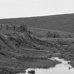
5. テスト画像の例
以下に各カテゴリのテスト画像の例を示す。
〜 MITforest 〜
 |
 |
〜 MITmountain 〜
 |
 |
〜 industrial 〜
 |
 |
〜 CALsuburb 〜
 |
 |
〜 MITopencountry 〜
 |
 |
2014年7月28日月曜日
gnuplotの図を保存する。
覚え書き
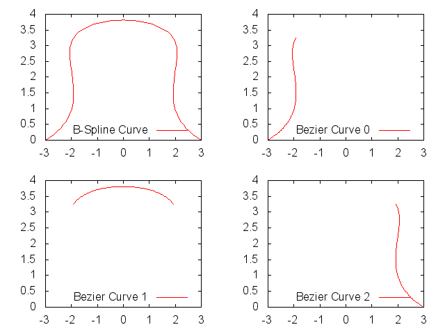
以下をdecompose_curve.pltとして保存し、 コマンドライン上で を実行すると、指定したディレクトリにこんなpng画像が保存される。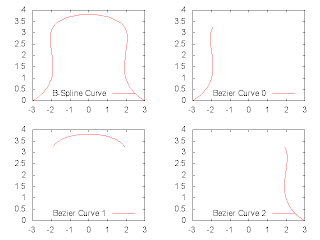 同様に以下をdecompose_surface.pltとして保存し、
以下を実行すると、
こんな画像が保存される。
同様に以下をdecompose_surface.pltとして保存し、
以下を実行すると、
こんな画像が保存される。
 曲面をグリッドにするには、こんなフォーマットでファイルを作る。
つまり、
曲面をグリッドにするには、こんなフォーマットでファイルを作る。
つまり、

以下をdecompose_curve.pltとして保存し、 コマンドライン上で を実行すると、指定したディレクトリにこんなpng画像が保存される。
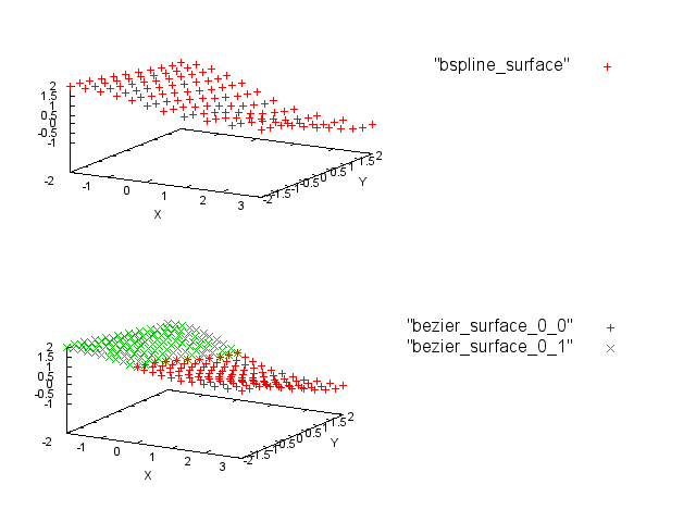
- データを、空行を使って、ブロックに分ける。
- 各ブロックはX座標あるいはY座標が同じである。

2014年7月27日日曜日
Coates's Method
in Japanese
In recent years a considerable number of studies have been made on the deep learning. The study by A. Coates et al. [1] focused on the reason why the deep learning achieves high performance. I have implemented their algorithm and applied it to the dataset I have at hand. In this page, I will provide a detailed explanation on their algorithm and show my results.
To realize the Coates's method, three datasets are needed:
The $K$-means clustering is applied to $M$ $N$-dimensional vectors. I have fully explained the clustering in this page. $K$ centroids are obtained.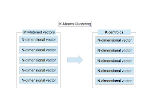 The image shown below indicates 961 centroids when $K=1000$ and $w=6$. To draw the image, after the elements of each vector are scaled so that they stay within the range of [0,255], the vector is converted to a 6$\times$6 image.

At this point, the following quantities are obtained:
Next the following procedures are conducted to the dataset $S_{\rm training}$.
 In the Coates's method, both the patch extraction and the pooling are executed only once. Moreover, the mapping function $f_{k}$ is computed using the unsupervised learning algorithm ($K$-means clustering). This is why the title of their paper is "Single-Layer Networks in Unsupervised Feature Learning."
Finally, the following procedures are conducted to the dataset $S_{\rm test}$.
I have implemented the algorithm in C++ and used the following libraries:
I have used the dataset called LSP15. It can be downloaded by clicking the title "scene category dataset" on this site. It has indoor and outdoor images that are classified into 15 categories. The number of images in each category is about 200 to 300, and image size is approximately 300$\times$300 pixels.
I have selected two categories and constructed four datasets $S_{\rm training}^{A/B}$ and $S_{\rm test}^{A/B}$.
The name of the image has an integer value like "image_0001.jpg." The integer value in the above table except for labels indicates the image name. The number of the training images and the test images are 150 and 50, respectively. The dataset used for making the feature mapping function $f_{k}$ is $S_{\rm unsupervised}=S_{\rm training}^{A} + S_{\rm training}^{B}$ which contains 300 images. Since the dataset includes 3-channel images (color images), they are converted to the gray images.
I have chosen the following parameters:
$\epsilon_{\rm w}$ is a small value to avoid divide-by-zero in the whitening matrix $M_{\rm W}$ defined by \begin{equation} M_{\rm W}=R\;\left(\Lambda+\epsilon_{\rm w}I\right)^{-1/2}\;R^{T}, \label{eq7} \end{equation} where $I$ is the identity matrix. I have already described the detailed explanation on the whitening here.
The results are shown below:
The Hellinger Kernel is able to be introduced by using the linear SVM after computing the square root of the element of the feature vector (Homogeneous Kernel Map).
An Analysis of Single-Layer Networks in Unsupervised Feature Learning, A. Coates, H. Lee, and A. Y. Ng, 2010
1. Introduction
In recent years a considerable number of studies have been made on the deep learning. The study by A. Coates et al. [1] focused on the reason why the deep learning achieves high performance. I have implemented their algorithm and applied it to the dataset I have at hand. In this page, I will provide a detailed explanation on their algorithm and show my results.
2. Algorithm
To realize the Coates's method, three datasets are needed:
- $S_{\rm unsupervised}$ : a dataset to construct the function which maps an image patch to a feature vector
- $S_{\rm training}$ : a dataset to train the Support Vector Machine (SVM)
- $S_{\rm test}$ : a dataset to test the SVM
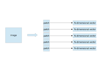
〜 Random Extraction of Patches 〜
- Extract randomly $n$ patches of $w \times w$ pixels from an image.
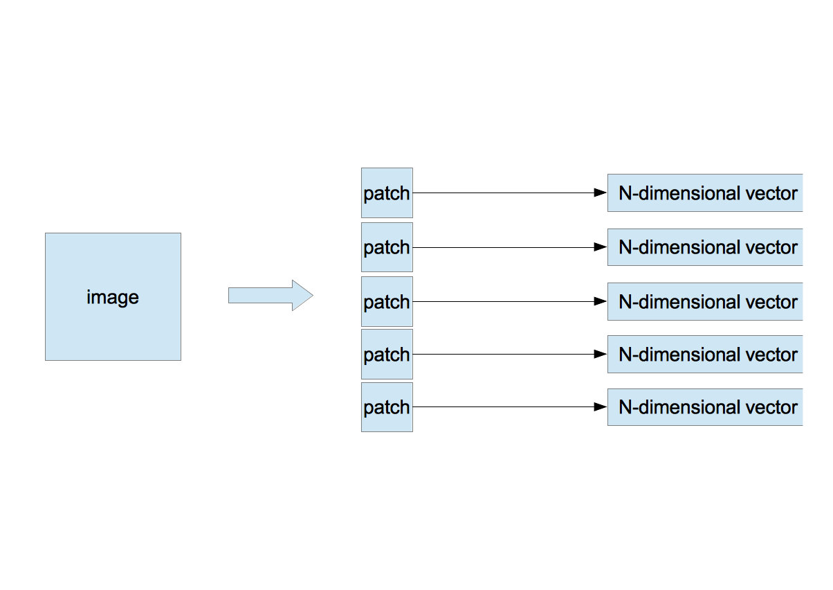
- Arrange pixels in a row from the left-top pixel to the right-bottom one of the patch to make a $N$-dimensional vector $\vec{x}$, where $N=d\times w\times w$ and $d$ is the number of channels. $d=3$ if the patch is color and $d=1$ if it is gray. As in my study the color image is converted to the gray one, $d$ is always 1.
- If there are $m$ images, the number of $N$-dimensional vectors is $M(=n\times m)$ as \begin{equation} \vec{x}^{\;\mu}, \mu=1,\cdots,M \end{equation}
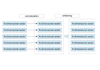
〜 Normalization and Whitening 〜
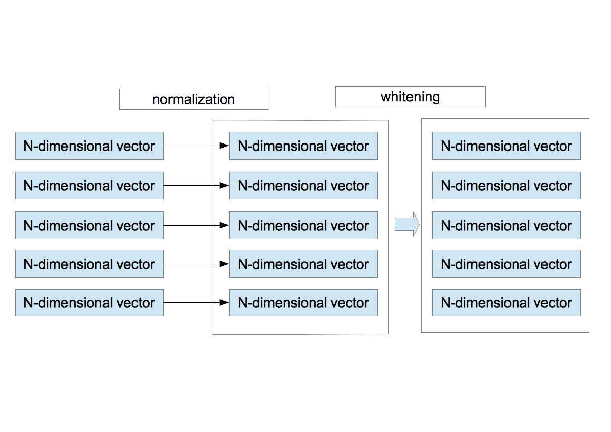
- For each vector $\vec{x}^{\;\mu}$, the average and the variance are calculated as \begin{eqnarray} \bar{x}^{\mu}&=&\frac{1}{N}\sum_{i=1}^{N}x_{i}^{\mu} \nonumber \\ \sigma_{\mu}^2 &=& \frac{1}{N}\sum_{i=1}^{N}\left(x_{i}^{\mu} - \bar{x}^{\mu}\right)^{2}. \nonumber \end{eqnarray} Using them, $\vec{x}^{\;\mu}$ is redefined by \begin{equation} x_{i}^{\mu} = \frac{x_{i}^{\mu} - \bar{x}^{\mu} }{ \sqrt{ \sigma_{\mu}^{2}+\epsilon_{\rm n} } }, \end{equation} where $\epsilon_{\rm n}$ is a small value to avoid divide-by-zero. This procedure corresponds to the brightness and contrast normalization of the local area.
- After normalizing $M$ vectors, they are whitened. Here is the detailed explanation on the whitening.
〜 Clustering 〜
The $K$-means clustering is applied to $M$ $N$-dimensional vectors. I have fully explained the clustering in this page. $K$ centroids are obtained.


〜 Mapping to Feature Vector 〜
At this point, the following quantities are obtained:
- The whitening matrix, $M_{\rm W}$
- $K$ centroids, $\vec{c}_{\;k}, k=1,\cdots,K$.
- Arrange pixels in a row from the left-top pixel to the right-bottom one of a path to make a $N$-dimensional vector $\vec{x}$.
- Normalize the vector $\vec{x}$.
- Whiten the normalized vector as $\vec{x}_{\rm W} = M_{\rm W}\;\vec{x}$
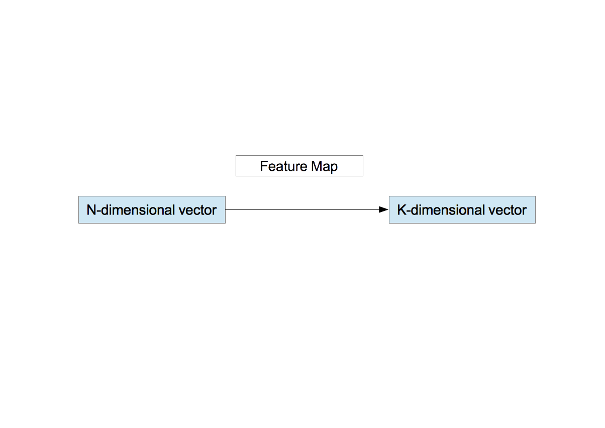
- Define the function $f_{k}(\vec{x}_{\rm W})$ as \begin{equation} f_{k}(\vec{x}_{\rm W})=\max{\left(0, \mu(z)-z_k\right)}, \nonumber \end{equation} where \begin{eqnarray} z_k&=&\|\vec{x}_{\rm W}-\vec{c}_{k} \| \nonumber \\ \mu(z)&=&\frac{1}{K}\sum_{k=1}^{K}z_k. \nonumber \end{eqnarray} $\mu(z)$ is the average distance between the vector $\vec{x}_{\rm W}$ and the $K$ centroids. The function $f_{k}$ outputs 0 if the distance $z_{k}$ between $\vec{x}_{\rm W}$ and the $k$-th centroid $\vec{c}_{k}$ is greater than the average $\mu(z)$ and outputs the finite value $\mu(z) - z_{k}$ if $z_{k}$ is less than $\mu(z)$. In other words in the context of the centroid images shown above, the function $f_{k}$ represents a degree of contribution of $K$ centroids to a patch. The function $f_{k}$ maps a $N$-dimensional vector to a $K$-dimensional vector. This is the feature vector.
Next the following procedures are conducted to the dataset $S_{\rm training}$.
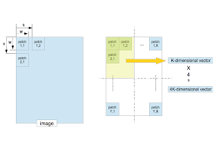
〜 Extraction of Feature Vectors From Training Images〜
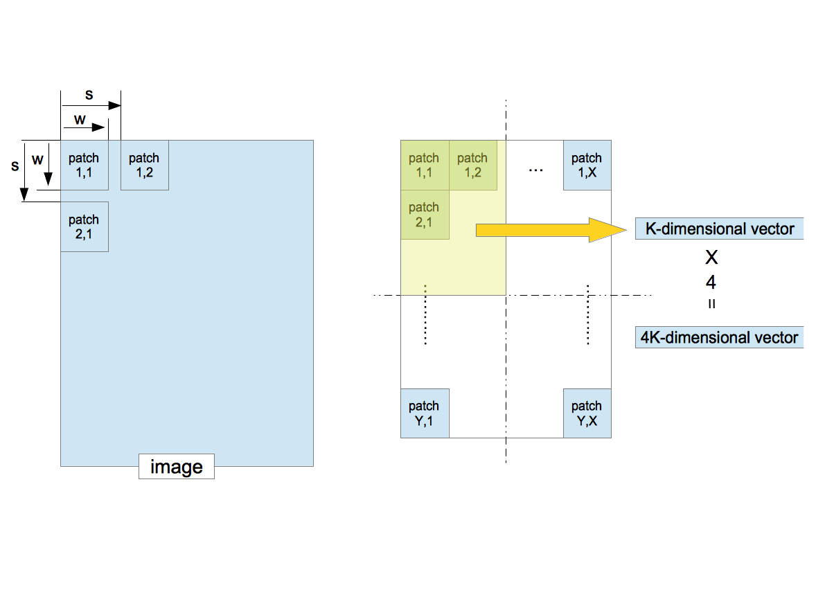
- Suppose that one image is given. The patches of $w\times w$ pixels are sequentially extracted from the image with the step size $s$ (stride).
- Convert a patch to a $K$-dimensional vector.
- The entire region which consists of all extracted patches is split into four equal-sized quadrants. Compute the average of the feature vectors in each quadrant. This procedure corresponds to the pooling in the deep learning. It not only decreases the location-dependency but also reduces the dimensionality of the feature vector.
- The four $K$-dimensional vectors yields a $4K$-dimensional vector. This is the feature vector made from one image. It is used for the classification by the SVM.
- If there are $D$ images, the number of $4K$-dimensional feature vectors is $D$.
- Train the SVM by using them.
Finally, the following procedures are conducted to the dataset $S_{\rm test}$.
〜 Classification of Test Dataset 〜
- Convert a given image to a $4K$-dimensional feature vector.
- Classify it by the SVM.
3. Implementation
I have implemented the algorithm in C++ and used the following libraries:
- opencv2: in order to implement procedures related to the image processing and the $K$-means clustering.
- boost::numeric::ublas: in order to implement the whitening computation.
- liblinear: in order to train SVM and classify images.
4. Image Dataset
I have used the dataset called LSP15. It can be downloaded by clicking the title "scene category dataset" on this site. It has indoor and outdoor images that are classified into 15 categories. The number of images in each category is about 200 to 300, and image size is approximately 300$\times$300 pixels.
I have selected two categories and constructed four datasets $S_{\rm training}^{A/B}$ and $S_{\rm test}^{A/B}$.
| category | training | test | label |
|---|---|---|---|
| A | 1-150 ($S_{\rm training}^{A}$) | 151-200 ($S_{\rm test}^{A}$) | -1 |
| B | 1-150 ($S_{\rm training}^{B}$) | 151-200 ($S_{\rm test}^{B}$) | +1 |
The name of the image has an integer value like "image_0001.jpg." The integer value in the above table except for labels indicates the image name. The number of the training images and the test images are 150 and 50, respectively. The dataset used for making the feature mapping function $f_{k}$ is $S_{\rm unsupervised}=S_{\rm training}^{A} + S_{\rm training}^{B}$ which contains 300 images. Since the dataset includes 3-channel images (color images), they are converted to the gray images.
5. Parameters
I have chosen the following parameters:
| $n$ | $w$ | $s$ | $K$ | $\epsilon_{\rm n}$ | $\epsilon_{\rm w}$ |
|---|---|---|---|---|---|
| 50 | 6 | 1 | 1000 | 10 | 0.1 |
$\epsilon_{\rm w}$ is a small value to avoid divide-by-zero in the whitening matrix $M_{\rm W}$ defined by \begin{equation} M_{\rm W}=R\;\left(\Lambda+\epsilon_{\rm w}I\right)^{-1/2}\;R^{T}, \label{eq7} \end{equation} where $I$ is the identity matrix. I have already described the detailed explanation on the whitening here.
6. Accuracy
The results are shown below:
| category A | category B | accuracy | accuracy(Hellinger Kernel) |
|---|---|---|---|
| bedroom | CALsuburb | 99%(99/100) | 97%(97/100) |
| livingroom | industrial | 94%(94/100) | 97%(97/100) |
| MITforest | MITmountain | 81%(81/100) | 86%(86/100) |
| industrial | CALsuburb | 88%(88/100) | 97%(97/100) |
The Hellinger Kernel is able to be introduced by using the linear SVM after computing the square root of the element of the feature vector (Homogeneous Kernel Map).
7. Discussion
- The accuracies are high in despite of the linear SVM.
- The Hellinger Kernel is effective except for the pair of bedroom and CALsuburb.
- The accuracy of the pair of MITforest and MITmountain is low compared with other pairs. If you see the sample images as shown below, it turns out that the images of the two categories are similar.
- The high performance is achieved without the commonly-used local feature algorithms, e.g. SIFT, SURF, BRIST, and so on. Will the study on them fade out?
〜 bedroom 〜
 |
 |
〜 livingroom 〜
 |
 |
〜 MITforest 〜
|
|
|
〜 industrial 〜
|
|
|
〜 MITmountain 〜
|
|
|
〜 CALsuburb 〜
|
|
|
8. References
2014年7月23日水曜日
Coatesの方法
in English
近年、Deep Learning の研究が盛んである。その中にはその高精度の原因を解明しようする研究もある。そのひとつが A.Coates らの "An Analysis of Single-Layer Networks in Unsupervised Feature Learning" である。今回これを実装し手元にある画像に適用してみたのでまとめます。
このアルゴリズムを検証するには、3つの画像セットが必要である。
最初に、$S_{\rm unsupervised}$ を使用して以下を行う。
$M$ 個の $N$ 次元ベクトルに対し、$K$-meansクラスタリングを行う。クラスタリングの手順はここにまとめてある。$K$ 個の重心が求まる。
下の画像は $K=1000$ としたときの961個の重心ベクトル($N=36$次元ベクトル)を画像化したものである(成分の最小値を0に最大値を255に置き換え6$\times$6の画像に変換した)。
ここまでの手順で以下のものが取得できた。
次に、$S_{\rm training}$ に対し以下を行う。
上の図を見れば明らかであるが、本手法はパッチの走査とPoolingがそれぞれ一度だけ行われる。また、パッチを特徴ベクトルへ変換する関数 $f_k$ は教師なし学習($K$-meansクラスタリング)により得られる。よって、Single-Layer Networks in Unsupervised Feature Learning なのである。
最後に、$S_{\rm test}$ に対し以下を行う。
実装言語はC++、使用したライブラリは以下の通りである。
使用した画像セットはLSP15と呼ばれているものである。ここの scene category dataset という項目をクリックするとダウンロードできる。15個のカテゴリに分類された室内・室外画像である。各カテゴリには、縦横200から300ピクセル程度の画像が200から300枚ほど含まれている。
今回の検証では、15個のカテゴリから適当に2つを選択し、画像セット $S_{\rm training}^{A/B}$、$S_{\rm test}^{A/B}$ を構成した。
ダウンロードした画像にはimage_0001.jpgのような番号を含む名前が付けられている。上の表の番号はこれを表す。 訓練画像は各カテゴリから150枚、テスト画像は50枚を選択した。 また、関数 $f_{k}$ を作るための画像セット $S_{\rm unsupervised}$は、$S_{\rm training}^{A} + S_{\rm training}^{B}$ とした。総数は300枚である。画像セットにはカラー画像も混ざっているが全てグレー画像に変換して検証を行った。
各種パラメータの値は以下の通りである。
ここで、$\epsilon_{\rm w}$ は白色化行列 $M_{\rm W}$ の0割りを防ぐ微小量である。 \begin{equation} M_{\rm W}=R\;\left(\Lambda+\epsilon_{\rm w}I\right)^{-1/2}\;R^{T} \label{eq7} \end{equation} ただし、$I$ は単位行列である。白色化行列の詳細はここにまとめてある。
結果を以下に示す。accuracyは通常の線形SVMを、accuracy(Hellinger Kernel)はHellinger Kernelを使用したときの識別率である。
Hellinger Kernelは、特徴ベクトルの各成分の平方根を計算したあと線形SVMを適用すれば実現できる(Homogeneous Kernel Map)。
1. はじめに
近年、Deep Learning の研究が盛んである。その中にはその高精度の原因を解明しようする研究もある。そのひとつが A.Coates らの "An Analysis of Single-Layer Networks in Unsupervised Feature Learning" である。今回これを実装し手元にある画像に適用してみたのでまとめます。
2. アルゴリズム
このアルゴリズムを検証するには、3つの画像セットが必要である。
- 特徴ベクトルを生成する関数を作るための画像セット($S_{\rm unsupervised}$)
- 訓練用画像セット($S_{\rm training}$)
- テスト用画像セット($S_{\rm test}$)
最初に、$S_{\rm unsupervised}$ を使用して以下を行う。
〜 パッチの切り出し 〜
- 1枚の画像からサイズ $w \times w$ のパッチをランダムに $n$ 枚切り出す。
- 1つのパッチの画素を左上から右下に向かって1列に並べ、$N$ 次元のベクトル $\vec{x}$ を作る。ここで $N=d\times w \times w$、$d$ は画像のチャンネル数である。カラー画像なら3、グレイ画像なら1である。
- 複数枚の画像について同じことを繰り返す。画像が $m$ 枚あれば $N$ 次元ベクトルは $M(=n\times m)$ 個作られる( $\vec{x}^{\;\mu}, \mu=1,\cdots,M$ )。
〜 正規化と白色化 〜
- 現在、$M$ 個の$N$ 次元ベクトルがある。個々のベクトルに対し、その成分の平均値と分散を計算し、正規化を行う。 \begin{eqnarray} \bar{x}^{\mu}&=&\frac{1}{N}\sum_{i=1}^{N}x_{i}^{\mu} \nonumber \\ \sigma_{\mu}^2 &=& \frac{1}{N}\sum_{i=1}^{N}\left(x_{i}^{\mu} - \bar{x}^{\mu}\right)^{2} \nonumber \end{eqnarray} これらを使って、改めて $\vec{x}^{\;\mu}$ を定義し直す。 \begin{equation} x_{i}^{\mu} = \frac{x_{i}^{\mu} - \bar{x}^{\mu} }{ \sqrt{ \sigma_{\mu}^{2}+\epsilon_{\rm n} } } \end{equation} ここで、$\epsilon_{\rm n}$ は0割りを防ぐ微小量である。この作業は、局所領域(パッチ)内での明るさとコントラストの正規化に相当する。
- 正規化された $M$ 個のベクトルを使って、白色化を行う。白色化の手順はここにまとめてある。
〜 クラスタリング 〜
$M$ 個の $N$ 次元ベクトルに対し、$K$-meansクラスタリングを行う。クラスタリングの手順はここにまとめてある。$K$ 個の重心が求まる。
〜 特徴ベクトルの作成 〜
ここまでの手順で以下のものが取得できた。
- 白色化行列 $M_{\rm W}$
- $K$ 個の重心座標 $\vec{c}_{\;k}, k=1,\cdots,K$
- パッチの画素を左上から右下に向かって1列に並べ、$N$ 次元のベクトル $\vec{x}$ を作成する。
- $\vec{x}$ を正規化する。
- 正規化した $\vec{x}$ に白色化行列 $M_{\rm W}$ をかけて白色化する。$\vec{x}_{\rm W} = M_{\rm W}\;\vec{x}$
- 関数 $f_{k}(\vec{x}_{\rm W})$ を次式で定義する。 \begin{equation} f_{k}(\vec{x}_{\rm W})=\max{\left(0, \mu(z)-z_k\right)} \nonumber \end{equation} ここで、 \begin{eqnarray} z_k&=&\|\vec{x}_{\rm W}-\vec{c}_{\;k} \| \nonumber \\ \mu(z)&=&\frac{1}{K}\sum_{k=1}^{K}z_k \nonumber \end{eqnarray} である。つまり、ある点 $\vec{x}_{\rm W}$ に注目したとき、この点と $K$ 個の重心との平均距離を算出する。 そして、平均距離より近い重心のインデックスには有限値を、遠い重心のインデックスには0を割り振る。 上の重心画像を使ってもう少し言い換えると、個々のパッチに対する各重心画像の寄与の度合いを表していることになる。 関数 $f_{k}$ により $N$ 次元ベクトルは、$K$ 次元ベクトルに変換される。これが特徴ベクトルである。
次に、$S_{\rm training}$ に対し以下を行う。
〜 訓練画像からの特徴ベクトルの抽出〜
- 1枚の訓練画像を考える。サイズ $w\times w$ のパッチを切り出す。その際、次のパッチとの距離(ストライド)を $s$ とする。左上から右下に向かって規則正しくパッチを取り出す。
- 各パッチから $K$ 次元の特徴ベクトルを算出する。
- 取り出したパッチが作る全領域を4等分し、各矩形に属する特徴ベクトルの平均ベクトルを計算する。この作業は、Deep LearningにおけるPoolingに相当する。識別対象の位置依存性を減らす手続きでもある。
- 4つの $K$ 次元ベクトルを並べた4 $K$ 次元ベクトルを、画像1枚に対する特徴ベクトルとする。
- 全ての訓練画像に対し同じことを繰り返す。訓練画像が $D$ 枚あれば、$D$ 個の4 $K$ 次元ベクトルが作られる。
- これらを使って、SVMで訓練する。
最後に、$S_{\rm test}$ に対し以下を行う。
〜 テスト画像の評価 〜
- 上と全く同じ手順で1枚の画像を4 $K$ 次元の特徴ベクトルに変換する。
- SVMで識別する。
3. 実装
実装言語はC++、使用したライブラリは以下の通りである。
- opencv2: 画像周りや $K$-meansクラスタリングなど。
- boost::numeric::ublas: 白色化の計算など。
- liblinear: 線形SVMを使った訓練とテスト。
4. 画像セット
使用した画像セットはLSP15と呼ばれているものである。ここの scene category dataset という項目をクリックするとダウンロードできる。15個のカテゴリに分類された室内・室外画像である。各カテゴリには、縦横200から300ピクセル程度の画像が200から300枚ほど含まれている。
今回の検証では、15個のカテゴリから適当に2つを選択し、画像セット $S_{\rm training}^{A/B}$、$S_{\rm test}^{A/B}$ を構成した。
| category | training | test | label |
|---|---|---|---|
| A | 1-150 ($S_{\rm training}^{A}$) | 151-200 ($S_{\rm test}^{A}$) | -1 |
| B | 1-150 ($S_{\rm training}^{B}$) | 151-200 ($S_{\rm test}^{B}$) | +1 |
ダウンロードした画像にはimage_0001.jpgのような番号を含む名前が付けられている。上の表の番号はこれを表す。 訓練画像は各カテゴリから150枚、テスト画像は50枚を選択した。 また、関数 $f_{k}$ を作るための画像セット $S_{\rm unsupervised}$は、$S_{\rm training}^{A} + S_{\rm training}^{B}$ とした。総数は300枚である。画像セットにはカラー画像も混ざっているが全てグレー画像に変換して検証を行った。
5. パラメータ
各種パラメータの値は以下の通りである。
| $n$ | $w$ | $s$ | $K$ | $\epsilon_{\rm n}$ | $\epsilon_{\rm w}$ |
|---|---|---|---|---|---|
| 50 | 6 | 1 | 1000 | 10 | 0.1 |
ここで、$\epsilon_{\rm w}$ は白色化行列 $M_{\rm W}$ の0割りを防ぐ微小量である。 \begin{equation} M_{\rm W}=R\;\left(\Lambda+\epsilon_{\rm w}I\right)^{-1/2}\;R^{T} \label{eq7} \end{equation} ただし、$I$ は単位行列である。白色化行列の詳細はここにまとめてある。
6. 識別率
結果を以下に示す。accuracyは通常の線形SVMを、accuracy(Hellinger Kernel)はHellinger Kernelを使用したときの識別率である。
| category A | category B | accuracy | accuracy(Hellinger Kernel) |
|---|---|---|---|
| bedroom | CALsuburb | 99%(99/100) | 97%(97/100) |
| livingroom | industrial | 94%(94/100) | 97%(97/100) |
| MITforest | MITmountain | 81%(81/100) | 86%(86/100) |
| industrial | CALsuburb | 88%(88/100) | 97%(97/100) |
Hellinger Kernelは、特徴ベクトルの各成分の平方根を計算したあと線形SVMを適用すれば実現できる(Homogeneous Kernel Map)。
7. 考察
- 線形SVMであるが全般的に識別率は高い。
- 1つを除いて、Hellinger Kernelの効果は高い。
- MITforestとMITmountainの組の識別率が他と比べて低いが、下のサンプル画像を見れば納得できると思う。
- 特別な局所特徴アルゴリズムを使わなくても高い識別率を達成できている。局所特徴アルゴリズムの研究は廃れていくのだろうか?
〜 bedroom 〜
|
|
|
〜 livingroom 〜
|
|
|
〜 MITforest 〜
|
|
|
〜 industrial 〜
|
|
|
〜 MITmountain 〜
|
|
|
〜 CALsuburb 〜
|
|
|
登録:
コメント (Atom)