memo: Coates's Method

1. Introduction

　In recent years a considerable number of studies have been made on the deep learning. The study by A. Coates et al. [1] focused on the reason why the deep learning achieves high performance. I have implemented their algorithm and applied it to the dataset I have at hand. In this page, I will provide a detailed explanation on their algorithm and show my results.

2. Algorithm

　To realize the Coates's method, three datasets are needed:

$S_{\rm unsupervised}$ : a dataset to construct the function which maps an image patch to a feature vector
$S_{\rm training}$ : a dataset to train the Support Vector Machine (SVM)
$S_{\rm test}$ : a dataset to test the SVM

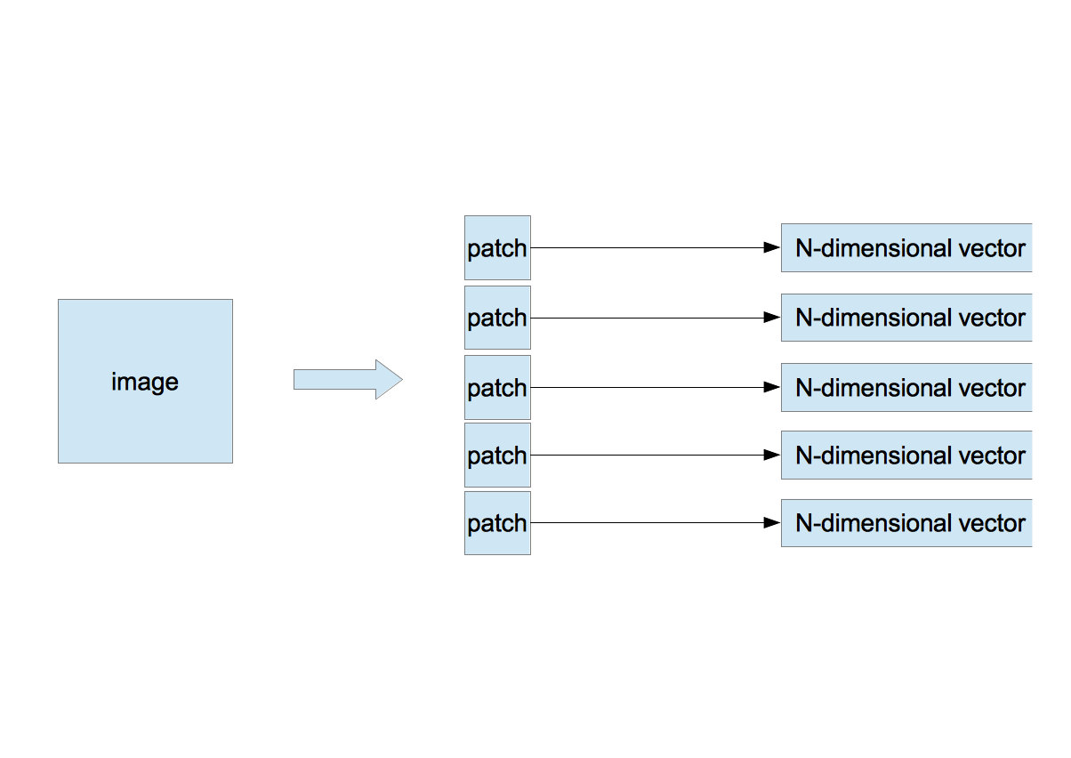
In my study, $S_{\rm unsupervised}$ and $S_{\rm training}$ are the same. First I conduct the following procedures to the dataset $S_{\rm unsupervised}$.

〜 Random Extraction of Patches 〜

Extract randomly $n$ patches of $w \times w$ pixels from an image.
Arrange pixels in a row from the left-top pixel to the right-bottom one of the patch to make a $N$-dimensional vector $\vec{x}$, where $N=d\times w\times w$ and $d$ is the number of channels. $d=3$ if the patch is color and $d=1$ if it is gray. As in my study the color image is converted to the gray one, $d$ is always 1.
If there are $m$ images, the number of $N$-dimensional vectors is $M(=n\times m)$ as \begin{equation} \vec{x}^{\;\mu}, \mu=1,\cdots,M \end{equation}

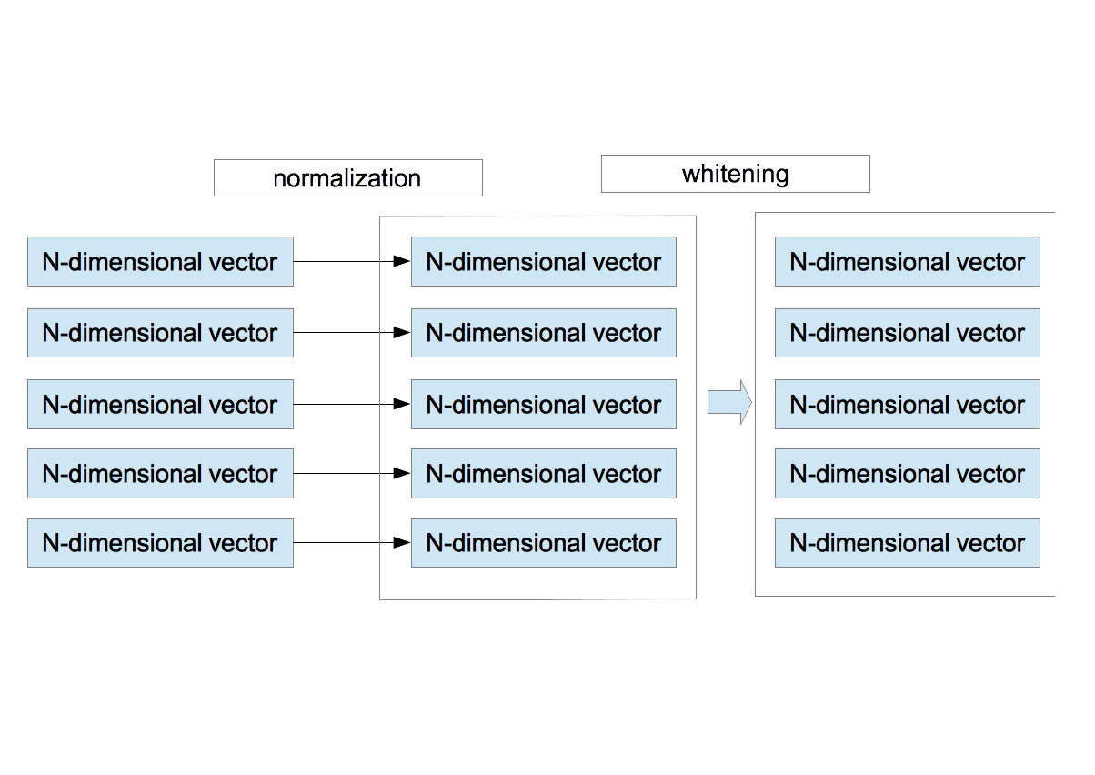
〜 Normalization and Whitening 〜

For each vector $\vec{x}^{\;\mu}$, the average and the variance are calculated as \begin{eqnarray} \bar{x}^{\mu}&=&\frac{1}{N}\sum_{i=1}^{N}x_{i}^{\mu} \nonumber \\ \sigma_{\mu}^2 &=& \frac{1}{N}\sum_{i=1}^{N}\left(x_{i}^{\mu} - \bar{x}^{\mu}\right)^{2}. \nonumber \end{eqnarray} Using them, $\vec{x}^{\;\mu}$ is redefined by \begin{equation} x_{i}^{\mu} = \frac{x_{i}^{\mu} - \bar{x}^{\mu} }{ \sqrt{ \sigma_{\mu}^{2}+\epsilon_{\rm n} } }, \end{equation} where $\epsilon_{\rm n}$ is a small value to avoid divide-by-zero. This procedure corresponds to the brightness and contrast normalization of the local area.
After normalizing $M$ vectors, they are whitened. Here is the detailed explanation on the whitening.

〜 Clustering 〜

　The $K$-means clustering is applied to $M$ $N$-dimensional vectors. I have fully explained the clustering in this page. $K$ centroids are obtained.

　The image shown below indicates 961 centroids when $K=1000$ and $w=6$. To draw the image, after the elements of each vector are scaled so that they stay within the range of [0,255], the vector is converted to a 6$\times$6 image.

〜 Mapping to Feature Vector 〜

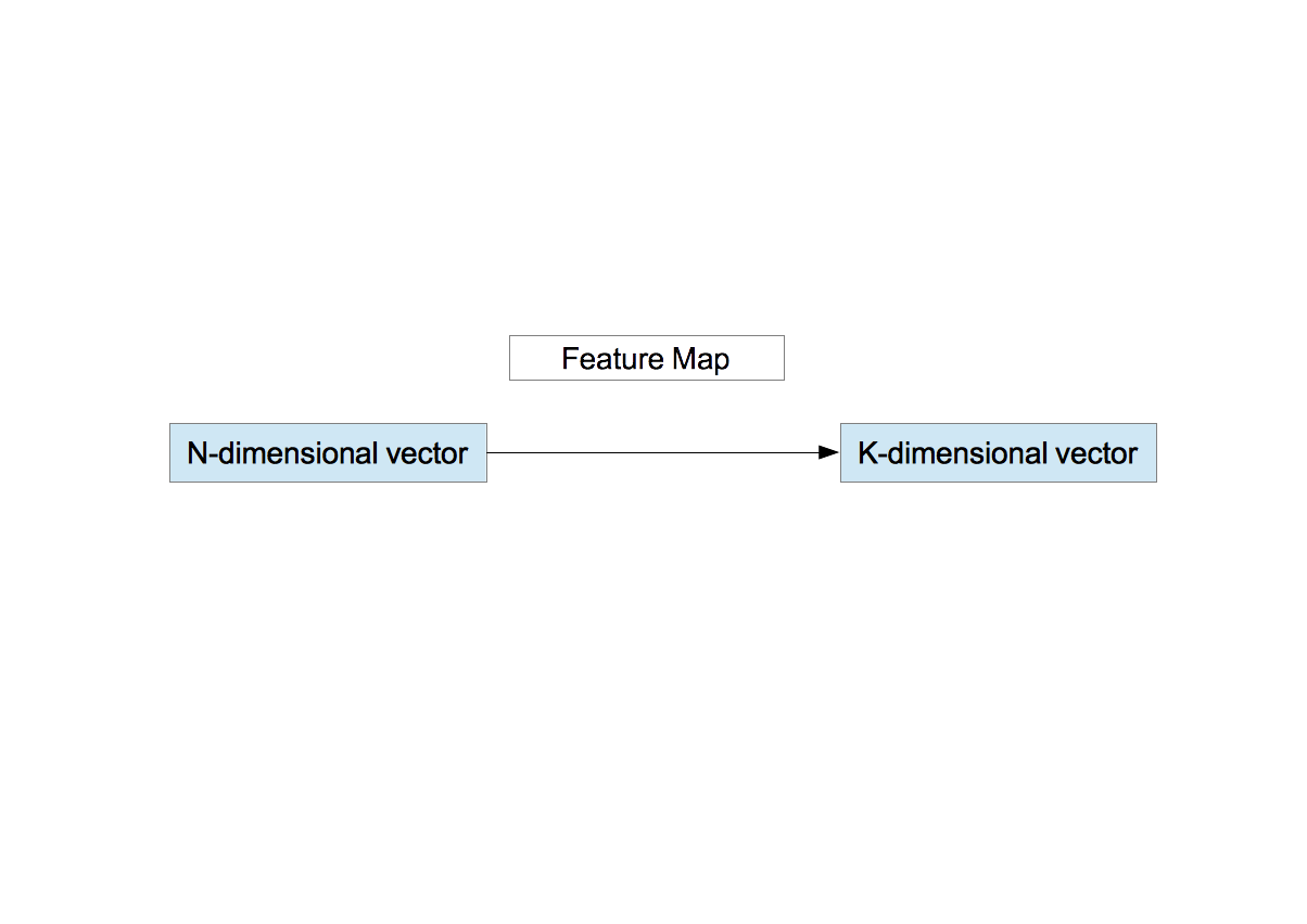
　At this point, the following quantities are obtained:

The whitening matrix, $M_{\rm W}$
$K$ centroids, $\vec{c}_{\;k}, k=1,\cdots,K$.

Using them, the function which maps a patch to a feature vector is constructed. The procedures are as follows:

Arrange pixels in a row from the left-top pixel to the right-bottom one of a path to make a $N$-dimensional vector $\vec{x}$.
Normalize the vector $\vec{x}$.
Whiten the normalized vector as $\vec{x}_{\rm W} = M_{\rm W}\;\vec{x}$
Define the function $f_{k}(\vec{x}_{\rm W})$ as \begin{equation} f_{k}(\vec{x}_{\rm W})=\max{\left(0, \mu(z)-z_k\right)}, \nonumber \end{equation} where \begin{eqnarray} z_k&=&\|\vec{x}_{\rm W}-\vec{c}_{k} \| \nonumber \\ \mu(z)&=&\frac{1}{K}\sum_{k=1}^{K}z_k. \nonumber \end{eqnarray} $\mu(z)$ is the average distance between the vector $\vec{x}_{\rm W}$ and the $K$ centroids. The function $f_{k}$ outputs 0 if the distance $z_{k}$ between $\vec{x}_{\rm W}$ and the $k$-th centroid $\vec{c}_{k}$ is greater than the average $\mu(z)$ and outputs the finite value $\mu(z) - z_{k}$ if $z_{k}$ is less than $\mu(z)$. In other words in the context of the centroid images shown above, the function $f_{k}$ represents a degree of contribution of $K$ centroids to a patch. The function $f_{k}$ maps a $N$-dimensional vector to a $K$-dimensional vector. This is the feature vector.

Next the following procedures are conducted to the dataset $S_{\rm training}$.

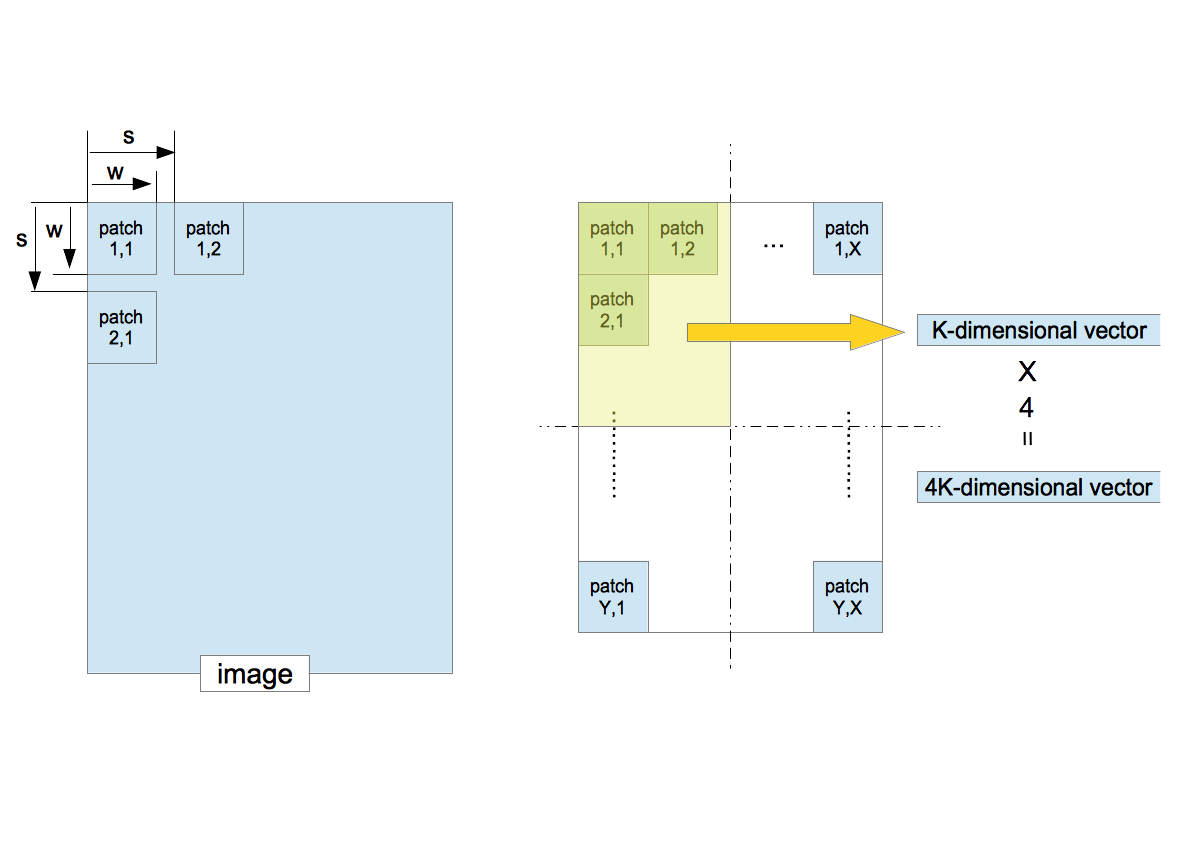
〜 Extraction of Feature Vectors From Training Images〜

Suppose that one image is given. The patches of $w\times w$ pixels are sequentially extracted from the image with the step size $s$ (stride).
Convert a patch to a $K$-dimensional vector.
The entire region which consists of all extracted patches is split into four equal-sized quadrants. Compute the average of the feature vectors in each quadrant. This procedure corresponds to the pooling in the deep learning. It not only decreases the location-dependency but also reduces the dimensionality of the feature vector.
The four $K$-dimensional vectors yields a $4K$-dimensional vector. This is the feature vector made from one image. It is used for the classification by the SVM.
If there are $D$ images, the number of $4K$-dimensional feature vectors is $D$.
Train the SVM by using them.

　In the Coates's method, both the patch extraction and the pooling are executed only once. Moreover, the mapping function $f_{k}$ is computed using the unsupervised learning algorithm ($K$-means clustering). This is why the title of their paper is "Single-Layer Networks in Unsupervised Feature Learning."

Finally, the following procedures are conducted to the dataset $S_{\rm test}$.

〜 Classification of Test Dataset 〜

Convert a given image to a $4K$-dimensional feature vector.
Classify it by the SVM.

3. Implementation

I have implemented the algorithm in C++ and used the following libraries:

opencv2: in order to implement procedures related to the image processing and the $K$-means clustering.
boost::numeric::ublas: in order to implement the whitening computation.
liblinear: in order to train SVM and classify images.

I have also used the python as a glue that binds procedures together.

4. Image Dataset

　I have used the dataset called LSP15. It can be downloaded by clicking the title "scene category dataset" on this site. It has indoor and outdoor images that are classified into 15 categories. The number of images in each category is about 200 to 300, and image size is approximately 300$\times$300 pixels.
　I have selected two categories and constructed four datasets $S_{\rm training}^{A/B}$ and $S_{\rm test}^{A/B}$.

category	training	test	label
A	1-150 ($S_{\rm training}^{A}$)	151-200 ($S_{\rm test}^{A}$)	-1
B	1-150 ($S_{\rm training}^{B}$)	151-200 ($S_{\rm test}^{B}$)	+1

The name of the image has an integer value like "image_0001.jpg." The integer value in the above table except for labels indicates the image name. The number of the training images and the test images are 150 and 50, respectively. The dataset used for making the feature mapping function $f_{k}$ is $S_{\rm unsupervised}=S_{\rm training}^{A} + S_{\rm training}^{B}$ which contains 300 images. Since the dataset includes 3-channel images (color images), they are converted to the gray images.

5. Parameters

　I have chosen the following parameters:

$n$	$w$	$s$	$K$	$\epsilon_{\rm n}$	$\epsilon_{\rm w}$
50	6	1	1000	10	0.1

$\epsilon_{\rm w}$ is a small value to avoid divide-by-zero in the whitening matrix $M_{\rm W}$ defined by \begin{equation} M_{\rm W}=R\;\left(\Lambda+\epsilon_{\rm w}I\right)^{-1/2}\;R^{T}, \label{eq7} \end{equation} where $I$ is the identity matrix. I have already described the detailed explanation on the whitening here.

6. Accuracy

　The results are shown below:

category A	category B	accuracy	accuracy(Hellinger Kernel)
bedroom	CALsuburb	99%(99/100)	97%(97/100)
livingroom	industrial	94%(94/100)	97%(97/100)
MITforest	MITmountain	81%(81/100)	86%(86/100)
industrial	CALsuburb	88%(88/100)	97%(97/100)

　The Hellinger Kernel is able to be introduced by using the linear SVM after computing the square root of the element of the feature vector (Homogeneous Kernel Map).

7. Discussion

The accuracies are high in despite of the linear SVM.
The Hellinger Kernel is effective except for the pair of bedroom and CALsuburb.
The accuracy of the pair of MITforest and MITmountain is low compared with other pairs. If you see the sample images as shown below, it turns out that the images of the two categories are similar.
The high performance is achieved without the commonly-used local feature algorithms, e.g. SIFT, SURF, BRIST, and so on. Will the study on them fade out?

　Two test images from each category are shown below: