Introduction
In the previous page, a scene recognition (15-class classification) was performed by using Chainer. In this page, a Fully Convolutional Network (FCN) is simplified and implemented by means of Chainer.
Computation Environment
The same instance as the previous page, g2.2xlarge in the Amazon EC2, is used.
Dataset
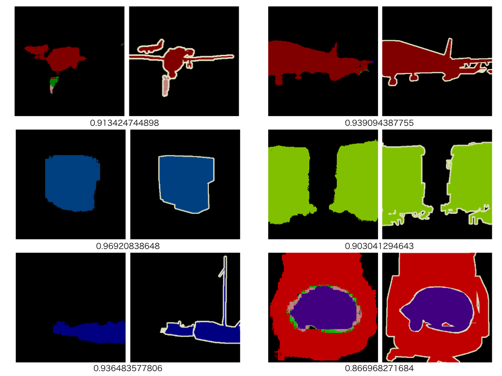
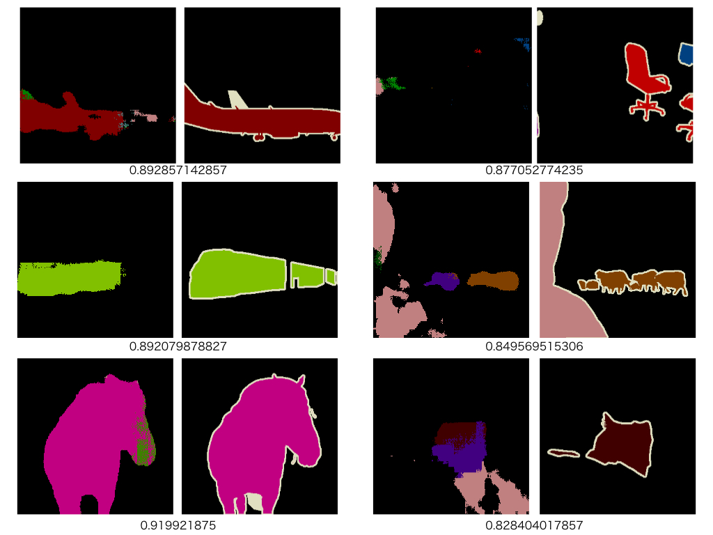
In this work an FCN is trained on a dataset VOC2012 which includes ground truth segmentations. The examples are given below:

| number of train | number of test |
|---|---|
| 2330 | 580 |
The number of the training (testing) images is rounded off to make it a multiple of 10 (5). 10 (5) is a mini batch size for the training (testing) images. Though the original FCN operates on an input of any size, for simplicity the FCN in this work takes a fixed-sized (224$\times$224) input. Therefore all images are resized in advance as shown below:

VOC2012 provides 21 classes as specified below:
| label | category |
|---|---|
| 0 | background | 1 | aeroplane | 2 | bicycle | 3 | bird | 4 | boat | 5 | bottle | 6 | bus | 7 | car | 8 | cat | 9 | chair | 10 | cow | 11 | diningtable | 12 | dog | 13 | horse | 14 | motorbike | 15 | person | 16 | potted plant | 17 | sheep | 18 | sofa | 19 | train | 20 | tv/monitor |
Network Structure
The detailed structure of a network used in this work is as follows:

pool5. For simplicity, these layers are removed in this work.
- name: a layer name
- input: a size of an input feature map
- in_channels: the number of input feature maps
- out_channels: the number of output feature maps
- ksize: a kernel size
- stride: a stride size
- pad: a padding size
- output: a size of an output feature map
pool3, pool4, and pool5 are followed by score-pool3, score-pool4, and score-pool5, respectively. Their parameters are shown below:

score-pool3, score-pool4, and score-pool5) outputs p3, p4, and p5.

upsampled_pool4 and upsampled_pool5 shown in the table above, are applied to p4 and p5, respectively. After summing their (upsample_pool4 and upsample_pool5) outputs and p3, the sum is upsampled back to the original image size through the layer upsample_final shown in the table. This net structure corresponds to the FCN-8s described in the original FCN.
Implementation of Network
The network can be written in Chainer like this:
-- myfcn.py -- I assigned pixels on the borderline between objects and a background with a label of -1. To do so leads to no contribution from those pixels when calculating
softmax_cross_entropy (see the Chainer's specification for details). The function calculate_accuracy also throws away contribution from the pixels on the borderline. The function add is defined as:-- add.py --
Training
The script to train is as follows:
-- train.py -- -- mini_batch_loader.py --
I used
copy_model described in the page. The file VGGNet.py was downloaded from the page. The procedures expressed in the script train.py are as follows:
- make an instance of the type
MiniBatchLoader - make an instance of the type
VGGNet - make an instance of the type
MyFcn - copy parameters of the
VGGNetinstance to those ofMyFcnone - select MomentumSGD as an optimization algorithm
- run a loop to train the net
Results
Iterations are terminated at the 62nd epoch. The accuracies and the losses for the training and testing datasets are shown below.
-- Training Dataset --


-- Training Dataset --

-- Testing Dataset --

Hey, Thank you for sharing great article!!!
返信削除I found a mistake in function load_data of MiniBatchLoader. In following section :
img = cv2.imread(path)
if img is None:
raise RuntimeError("invalid image: {i}".format(i=path))
xs[i, :, :, :] = ((img - self.mean)/255).transpose(2, 0, 1)
I think image type must be float32 so,
'img = cv2.imread(path)'
should be
'img = cv2.imread(path).astype(np.float32)'
. What do you think?
Thank you for your comment.
削除I think that the automatic cast to float32 is executed by the following code:
xs[i, :, :, :] = ((img - self.mean)/255).transpose(2, 0, 1)
where self.mean is an array of float32.