3D Object Retrieval On SHREC2012 Dataset

Introduction

　In the previous page a new method for 3D object recognition which is based on the work by H. Su et al. is proposed and evaluated on two 3D object datasets of the ModelNet10 and the ModelNet40. The classification accuracies for them reach 92.84% and 90.92%, respectively. The method employs a convolutional neural network (CNN) as a feature extractor and a support vector machine (SVM) as a classifier. In this page 3D object retrieval on SHREC2012 dataset is performed using the feature extractor which is the part of the new method. It is demonstrated that Nearest Neighbor (NN), First-Tier (FT), Second-Tier (ST), F-Measure (F), and Discounted Cumulative Gain (DCG) are all better than those by the other studies shown in the page.

Dataset

　The SHREC2012 dataset consists of 60 categories each of which has 20 3D models that are in the ASCII Object File Format (*.off). The total number of the 3D models is 1200. In order to train the CNN, a set of 3D models in each category is divided by the split ratio 4:1. The former group corresponds to a training dataset in which the number of 3D models is 960. The latter one includes 240 3D models and is considered as a testing dataset. As explained here, in the proposed method 20 gray images are created per 3D object. Therefore, the numbers of the training and the testing images are 19200(=20$\times$960) and 4800(=20$\times$240), respectively. Since the vertical and the horizontal flipped images are added only to the training dataset, its number is finally 57600(=3$\times$19200).

the number of training images	the number of testing images
57600	4800

Algorithm

　The CNN model (bvlc_reference_caffenet.caffemodel) that Caffe provides is fine-tuned on the training dataset. The detailed information on the fine-tuning procedures is described in this page. The following figure shows a fine-tuning process.

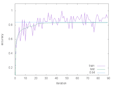
The x-axis indicates the iteration number and the y-axis the recognition accuracy. Because in my work the total iteration number is set to 59,000 and a solver file, where parameters for training are defined, is designed to output the accuracy once per 1000 iterations, the maximum value of the x-axis is 59(=59,000/1000). It can be seen that the recognition accuracy reaches about 78.9%.
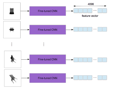
　After training, an output of the layer "fc7" is used as a feature vector (4096 dimensions). As explained here, in the proposed method a 3D object yields 20 gray images which are converted from depth ones. The fine-tuned CNN used as the feature extractor is applied to each of them and 20 feature vectors are obtained per 3D object.

According to the work by H. Su et al., the element-wise maximum operation across the 20 vectors is used to make a single feature vector with 4096 dimensions as shown below.

It is worthy of noting that one feature vector per 3D object is obtained.

Evaluation Measures

　Now that the feature extractor is constructed, five standard performance metrics, Nearest Neighbor (NN), First-Tier (FT), Second-Tier (ST), F-Measure (F), and Discounted Cumulative Gain (DCG), can be calculated by means of the evaluation code, SHREC2012_Generic_Evaluation.m, which is an m-file for MATLAB. The tables shown below compare the proposed method and the other studies. The latter results are quoted from the page.

Nearest Neighbor (NN)

Method	NN
LSD-sum	0.517
ZFDR	0.818
3DSP_L3_200_hik	0.708
DVD+DB	0.831
DG1SIFT	0.879
the proposed method	0.943

First-Tier (FT)

Method	FT
LSD-sum	0.232
ZFDR	0.491
3DSP_L2_1000_hik	0.376
DVD+DB+GMR	0.613
DG1SIFT	0.661
the proposed method	0.707

Second-Tier (ST)

Method	ST
LSD-sum	0.327
ZFDR	0.621
3DSP_L2_1000_hik	0.502
DVD+DB+GMR	0.739
DG1SIFT	0.799
the proposed method	0.827

F-Measure (F)

　I think that there is a mistake of understanding the F-Measure as the E-Measure in the page.
　

Method	F
LSD-sum	0.224
ZFDR	0.442
3DSP_L2_1000_hik	0.351
DVD+DB+GMR	0.527
DG1SIFT	0.576
the proposed method	0.599

Discounted Cumulative Gain (DCG)

　Accurately the ratio of DCG to Ideal Discounted Cumulative Gain (IDCG) is calculated.

Method	DCG/IDCG
LSD-sum	0.565
ZFDR	0.776
3DSP_L2_1000_hik	0.685
DVD+DB+GMR	0.833
DG1SIFT	0.871
the proposed method	0.905

Precision-Recall Curve (PR)

　Though the evaluation code does not support the PR, the other studies show it. In my work it is calculated by the following procedure.

1. Since one curve can be computed from one query, 1,200 curves are obtained.
2. After interpolating each curve within the range of [0, 1] with a step of 0.01, the average of a series of curves is calculated.

Average Precision (AP)

　This quantity which the other studies present is also not offered by the evaluation code. In my work, by defining the AP as the area under the precision-recall curve, it is calculated.

Method	AP
LSD-sum	0.381
ZFDR	0.650
3DSP_L2_1000_hik	0.526
DVD+DB+GMR	0.765
DG1SIFT	0.811
the proposed method	0.818

I don't know whether or not two quantities, PR and AP, are computed in exactly the same way as the other studies.

3D Object Recognition by CNN and SVM

Introduction

　A method for 3D object recognition, which is based on the work by H. Su et al., has been already proposed and evaluated on two 3D object datasets of the ModelNet10 and the ModelNet40. The classification accuracy for the ModelNet10 dataset has been shown here and that for the ModelNet40 dataset here. The method makes use of a convolutional neural network (CNN) as both a feature extractor and a classifier. In this page the method is extended to apply the CNN as only a feature extractor and to perform a classification by means of a support vector machine (SVM). It is demonstrated that the classification accuracy of the method is a little higher than those of the previous methods.

Classification Accuracies

　The following table shows classification accuracies for the previous and the proposed methods. The previous results are quoted from the Princeton ModelNet page.

Algorithm	Accuracy(ModelNet10)	Accuracy(ModelNet40)
MVCNN		90.1%
VoxNet	92%	80.3%
DeepPano	85.45%	77.63%
3DShapeNets	83.5%	77%
the proposed method	92.84%	90.92%

Proposed Method

　In the proposed method the CNN is used as a feature extractor and the SVM is applied as a classifier.

Feature Extractor:

　The CNN model (bvlc_reference_caffenet.caffemodel) that Caffe provides is fine-tuned on the training set of ModelNet10 or the ModelNet40. The detailed information on the fine-tuning procedures is described in this page. After training, output of the layer "fc7" is used as a feature vector (4096 dimensions). As explained here, in the proposed method a 3D object yields 20 gray images which are converted from depth ones. The fine-tuned CNN used as the feature extractor is applied to each of them and 20 feature vectors are obtained per 3D object.

According to the work by H. Su et al., element-wise maximum value across the 20 vectors is taken to make a single feature vector with 4096 dimensions as shown below.

Classifier:

　Since one feature vector per 3D object is made, it is straightforward to perform a classification by the SVM. In the current work the library LIBLINEAR in which linear SVMs are implemented is used. For the ModelNet10 training set the following command is run to train the SVM, and for the ModelNet40 training set the command is as follows, It is worthwhile to note that in order to improve the accuracy, square root of all elements of the vector is computed before applying the linear SVM. In other words, a Hellinger kernel classifier is employed. After training, the prediction command is run for the testing sets of both the ModelNet10 and the ModelNet40 as, The programs "train" and "predict" are offered by LIBLINEAR.

References

1. MVCNN: Hang Su, Subhransu Maji, Evangelos Kalogerakis, and Erik Learned-Miller, Multi-view Convolutional Neural Networks for 3D Shape Recognition
2. VoxNet: D. Maturana and S. Scherer. VoxNet: A 3D Convolutional Neural Network for Real-Time Object Recognition. IROS2015.
3. DeepPano: B Shi, S Bai, Z Zhou, X Bai. DeepPano: Deep Panoramic Representation for 3-D Shape Recognition. Signal Processing Letters 2015.
4. 3DShapeNets: Z. Wu, S. Song, A. Khosla, F. Yu, L. Zhang, X. Tang and J. Xiao. 3D ShapeNets: A Deep Representation for Volumetric Shapes. CVPR2015.

3D Object Recognition by Caffe 〜 40-class classification 〜

Introduction

　In the previous page, a new method for a 3D object recognition was proposed. The method is based on the work of H. Su et al. and was applied to a 10-class classification by means of the ModelNet10 dataset. A high classification accuracy of 90.2% was achieved. In this page, the method is evaluated on the ModelNet40 dataset. It is shown that a classification accuracy of 87.16% is reached.

Dataset

　The CNN model (bvlc_reference_caffenet.caffemodel) that Caffe provides is fine-tuned using the ModelNet40 dataset which consists of 40 categories. Each category has training and testing 3D models which are in Object File Format (OFF). The numbers of the models are as follows:

the number of trainings	the number of testing
9843	2468

Fine-tuning Result

　The following figure shows a fine-tuning process.

The x-axis indicates the iteration number and the y-axis the recognition accuracy. Because in the current case the total iteration number is 90,000 and the solver is designed to output the accuracy once per 1000 iterations, the maximum value of the x-axis is 90(=90,000/1000). It can be seen that the recognition accuracy reaches about 83.6%.

Classification Accuracy

　As described in the previous page, a 3D model yields 20 gray images. The fine-tuned CNN is applied to each of them and 20 labels are obtained per 3D model. The final label is decided by majority vote. This algorithm is evaluated on the 3D models belonging to the test phase . The number of them is 2468 as shown above. The classification accuracy reaches 87.16%(=2151/2468). The following table is quoted from the Princeton ModelNet page. The algorithm proposed here is not bad in spite of the simple procedures.

Algorithm	Accuracy
MVCNN	90.1%
VoxNet	80.3%
DeepPano	77.63%
3DShapeNets	77%
the proposed algorithm	87.16%

The detailed information on accuracy for each category is shown below.

References

1. Hang Su, Subhransu Maji, Evangelos Kalogerakis, and Erik Learned-Miller, Multi-view Convolutional Neural Networks for 3D Shape Recognition
2. D. Maturana and S. Scherer. VoxNet: A 3D Convolutional Neural Network for Real-Time Object Recognition. IROS2015.
3. B Shi, S Bai, Z Zhou, X Bai. DeepPano: Deep Panoramic Representation for 3-D Shape Recognition. Signal Processing Letters 2015.
4. Z. Wu, S. Song, A. Khosla, F. Yu, L. Zhang, X. Tang and J. Xiao. 3D ShapeNets: A Deep Representation for Volumetric Shapes. CVPR2015.

3D Object Recognition by Caffe 〜 20-class classification 〜

Introduction

　In the previous page, a new method for a 3D object recognition was proposed. The method was applied to a 10-class classification and a classification accuracy of 90.2% was achieved. In this page, the method is evaluated on a 20-class classification. It is shown that a high classification accuracy of 95.3% is reached.

Dataset

　The pre-trained CNN model (bvlc_reference_caffenet.caffemodel) that Caffe provides is fine-tuned using a dataset consisting of 20 categories which are chosen among the ModelNet40 dataset. These categories are shown below.

1. airplane
2. bathtub
3. bed
4. bench
5. bookshelf
6. bottle
7. bowl
8. car
9. chair
10. cone
11. cup
12. curtain
13. desk
14. door
15. dresser
16. flower_pot
17. glass_box
18. guitar
19. keyboard
20. lamp

Each category has training and testing 3D models which are in Object File Format (OFF). The numbers of the models in categories are as follows:

label	name	the number of trainings	the number of testings
0	airplane	626	100
1	bathtub	106	50
2	bed	515	100
3	bench	173	20
4	bookshelf	572	100
5	bottle	335	100
6	bowl	64	20
7	car	197	100
8	chair	889	100
9	cone	167	20
10	cup	79	20
11	curtain	138	20
12	desk	200	86
13	door	109	20
14	dresser	200	86
15	flower_pot	149	20
16	glass_box	171	100
17	guitar	155	100
18	keyboard	145	20
19	lamp	124	20
		5114	1202

Results of CNN and Classification

　The fine-tuning yields a high recognition accuracy of 93% as shown below.

As described in the previous page, a 3D model yields 20 gray images. The fine-tuned CNN is applied to each of them and 20 labels are obtained per 3D model. The final label is decided by majority vote. This algorithm is evaluated on those 3D models belonging to the test phase whose number is 1202 as shown above. The classification accuracy of 95.3% is reached.

my own memo: cpplinq

Sample code

Output

3D Object Recognition by Caffe

Introduction

　In this page, a 3D object recognition is performed by means of the library Caffe. The algorithm which is proposed here is based on the work of H. Su et al.. It is shown that with the pre-trained model that Caffe provides and its fine-tuning by the ModelNet10 dataset, the recognition accuracy achieves about 90.2% .

Computation Environment

　An instance "g2.2xlarge" in the Amazon EC2 is used. It mounts the GPU device on which the CUDA driver is installed.

Dataset

　The CNN model (bvlc_reference_caffenet.caffemodel) that Caffe provides is fine-tuned using the ModelNet10 dataset which consists of 10 categories as follows:

1. bathtub
2. bed
3. chair
4. desk
5. dresser
6. monitor
7. night stand
8. sofa
9. table
10. toilet

Each category has training and testing 3D models which are in Object File Format (OFF). The numbers of the models in categories are as follows:

label	name	the number of trainings	the number of testings
0	bathtub	106	50
1	bed	515	100
2	chair	889	100
3	desk	200	86
4	dresser	200	86
5	monitor	465	100
6	night stand	200	86
7	sofa	680	100
8	table	392	100
9	toilet	344	100
		3991	908

Training Algorithm

　The following procedures are applied to the training 3D models.

1. A 3D model is loaded.
2. It is scaled to such an appropriate size that all models have the same size.
3. The centroid is calculated.
4. A regular dodecahedron is placed centering around the centroid.
5. 20 depth images (400$\times$400 pixels) are drawn by making the 20 vertices of the dodecahedron view points.
6. The images are converted to gray images with the range [0,255].
7. The 20 gray images are obtained per model. Those images have the same label.
8. The pre-trained CNN model that Caffe provides is fine-tunued by them.

A regular dodecahedron placed centering around the centroid:

The 20 gray images converted from corresponding depth images:

It is worth noting that the number of the gray images which are inputs for the pre-trained CNN is 20 times as many as that of the 3D models.

	the number of trainings	the number of testings
3D model	3991	908
gray image ($\times$20)	79820	18160

Prediction Algorithm

　The following procedures are applied to the testing 3D models:

1. A 3D model is loaded.
2. It was scaled to such an appropriate size that all models have the same size.
3. The centroid is calculated.
4. A regular dodecahedron is placed centering around the centroid.
5. 20 depth images (400$\times$400 pixels) are drawn by making the 20 vertices of the dodecahedron view points.
6. The images are converted to gray images with the range [0,255].
7. The 20 gray images are obtained per model.
8. The above fine-tuned CNN is applied to the 20 gray images.
9. The 20 labels are obtained.
10. The resultant label is decided by majority vote.

Dataset for Caffe

　Caffe requires the following directories and files:

1. a directory which contains training images
2. a directory which contains testing images
3. a text file in which names and labels of training images are described
4. a text file in which names and labels of testing images are described

In this work they are referred to as "ModelNet10Train", "ModelNet10Test", "train.txt", and "test.txt,", respectively. The contents of "test.txt" are as follows:

desk_0234_depth_image_0.png 3
night_stand_0224_depth_image_0.png 6
chair_0904_depth_image_0.png 2
desk_0208_depth_image_0.png 3
bathtub_0127_depth_image_0.png 0
monitor_0528_depth_image_0.png 5
desk_0241_depth_image_0.png 3
dresser_0285_depth_image_0.png 4
sofa_0751_depth_image_0.png 7
dresser_0218_depth_image_0.png 4
....

The contents of "train.txt" are as follows:

chair_0190_depth_image_0.png 2
sofa_0138_depth_image_0.png 7
chair_0019_depth_image_0.png 2
dresser_0086_depth_image_0.png 4
table_0232_depth_image_0.png 8
sofa_0097_depth_image_0.png 7
night_stand_0040_depth_image_0.png 6
chair_0501_depth_image_0.png 2
chair_0766_depth_image_0.png 2
bed_0370_depth_image_0.png 1
...

After storing the images specified in "test.txt" and "train.txt" in the directories "ModelNet10Test" and "ModelNet10Train" respectively, this script is run to create a dataset for Caffe. "test_lmdb" and "train_lmdb" which are inputs for Caffe are output.

Definition of CNN

　The CNN model is defined in the file "train_val.prototxt" as The file is based on the file "bvlc_reference_caffenet/train_val.prototxt" that Caffe provides. The differences between the original and my own files exists in two layers, "data" and "fc8." In accordance with the interpretation in this page, parameters in the layer "3dobject_fc8" are modified as shown above.

Definition of Solver

　Based on the file "bvlc_reference_caffenet/solver.prototxt," the file used for fine-tuning the CNN is written as, The file is named "solver.prototxt."

Training

　This script is run to fine-tune the CNN model. The pre-trained model which Caffe provides is "bvlc_reference_caffenet/bvlc_reference_caffenet.caffemodel" which is passed to "caffe train" command as the argument of the "-weights." That script fine-tunes the pre-trained model by using the current dataset.

Result

　The x-axis indicates the iteration number and the y-axis the recognition accuracy. Because in the current case the total iteration number is 100,000 and the solver is designed to output the accuracy once per 1000 iterations, the maximum value of the x-axis is 100(=100,000/1000). The recognition accuracy reaches about 86%.

Construction of Classifier

　After training, a file "3dobject_train_iter_100000.caffemodel" is created. It is called a model file. The file contains the information on the fine-tuned CNN. In order to construct a classifier from the model file, the following file is also needed. That file is named "deploy.ptototxt." To get it, "train_val.prototxt" previously defined is modified according to the following procedures.

1. Remove the layer "data," and add following four lines.
2. Remove the layers "loss" and "accuracy", and add this layer.

The four lines with which the layer "data" is replaced means:

1. input_dim: 20 --- batch size
2. input_dim: 3 --- channel number
3. input_dim: 227 --- width of an image
4. input_dim: 227 --- height of an image

The code to classify the 3D models is implemented as follows: As described above, a 3D model yields 20 gray images. The fine-tuned CNN is applied to each of them and 20 labels are obtained per 3D model. The final label is decided by majority vote. This algorithm is evaluated on 3D models in the directory "ModelNet10Test." The number of them is 908 as shown above. The algorithm achieves 90.2% classification accuracy.

Comparison With Other Works

　The following table is quoted from the Princeton ModelNet page. The algorithm proposed here is not bad in spite of the simple procedures.

Algorithm	Accuracy
VoxNet	92%
DeepPano	85.45%
3DShapeNets	83.5%
the proposed algorithm	90.2%

References

1. D. Maturana and S. Scherer. VoxNet: A 3D Convolutional Neural Network for Real-Time Object Recognition. IROS2015.
2. B Shi, S Bai, Z Zhou, X Bai. DeepPano: Deep Panoramic Representation for 3-D Shape Recognition. Signal Processing Letters 2015.
3. Z. Wu, S. Song, A. Khosla, F. Yu, L. Zhang, X. Tang and J. Xiao. 3D ShapeNets: A Deep Representation for Volumetric Shapes. CVPR2015.
4. Hang Su, Subhransu Maji, Evangelos Kalogerakis, and Erik Learned-Miller, Multi-view Convolutional Neural Networks for 3D Shape Recognition

Feature Extraction by CNN and Classification by SVM

Introduction

　In the previous page, I performed the scene recognition using the Convolutional Neural Network (CNN) that the library Caffe provides. In this page, for the same dataset the same CNN is used for extracting feature vectors and the classification is accomplished by means of the Support Vector Machine (SVM) in the library LIBLINEAR. The recognition accuracy reaches about 95% .

Feature Extraction

　The following code is used to extract feature vectors from the CNN and to convert them into the input format that LIBLINEAR requires. The format of training and testing data files for LIBLINEAR is the same as that for LIBSVM: Each line contains a label and a feature vector. I extracted feature vectors from the layer "fc7." Their dimension is 4096. The contents of the file "total_list_15_in_local_machine.txt" described in the above code are as follows: Each line consists of a file path, a label, and a phase ("train"/"valid"/"test"). In this work, two phases "train" and "valid" are merged into one phase "train." After executing the above python code, I got two files "libsvm_train_inputs.txt" and "libsvm_test_inputs.txt" which are input files for LIBLINEAR. The number of training images are 7560 and the number of testing images 1220.

Execution of SVM

　The following command is run to train a SVM. Then, this command is run to predict the categories. The recognition accuracy is about as much as that of the CNN.

Scene Recognition by Caffe

Introduction

　In this page, I perform a scene recognition by means of the library Caffe. It is shown that with the pre-training model that Caffe provides and its fine-tuning by scene images, the recognition accuracy achieves about 95% .

Computation Environment

　I used that instance g2.2xlarge in the Amazon EC2 which mounts the GPU device.

Dataset

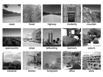
　I trained the CNN using the dataset LSP15 in this page. The dataset consists of the 15 directories as follows:

1. MITcoast
2. MITforest
3. MIThighway
4. MITinsidecity
5. MITmountain
6. MITopencountry
7. MITstreet
8. MITtallbuilding
9. bedroom
10. CALsuburb
11. industrial
12. kitchen
13. livingroom
14. PARoffice
15. store

The name of the directory represents the category of the scene. Each directory contains about 200 to 300 images which belong to their category.

Data Augmentation

　In order to augment dataset, I added the mirror images to it. Moreover, the images are split into two groups "train" and "test." The size of the image is 256 $\times$ 256, and the number of the channel is 3. The number of the images in each category is as follows:
　 　 　 　 　 　 　 　 　 　 　 　 　 　 　 　 　 　

label	name	number of train	number of test
0	MITcoast	610	100
1	MIThighway	440	70
2	MITmountain	630	100
3	MITstreet	490	80
4	MITforest	550	90
5	MITinsidecity	520	80
6	MITopencountry	690	110
7	MITtallbuilding	600	100
8	bedroom	360	60
9	CALsuburb	400	60
10	industrial	520	80
11	kitchen	360	60
12	livingroom	490	80
13	PARoffice	360	60
14	store	540	90
		7560	1220

Dataset for Caffe

　Caffe requires the following directories and files:

1. a directory which contains training images
2. a directory which contains test images
3. a text file in which names and labels of training images are described
4. a text file in which names and labels of test images are described

In my environment, they are put in the following paths:

1. /home/ubuntu/data/caffe_256_15/train/
2. /home/ubuntu/data/caffe_256_15/test/
3. /home/ubuntu/data/caffe_256_15/train.txt
4. /home/ubuntu/data/caffe_256_15/test.txt

The contents of the file "test.txt" are as follows:

MITstreet_image_0179_flipped.jpg 3
MITtallbuilding_image_0173_flipped.jpg 7
MITcoast_image_0126.jpg 0
store_image_0158_flipped.jpg 14
MITinsidecity_image_0102_flipped.jpg 5
MITforest_image_0200_flipped.jpg 4
industrial_image_0189_flipped.jpg 10
MITcoast_image_0142.jpg 0
kitchen_image_0019_flipped.jpg 11
bedroom_image_0210_flipped.jpg 8
bedroom_image_0116_flipped.jpg 8
livingroom_image_0008_flipped.jpg 12
kitchen_image_0051_flipped.jpg 11
MITstreet_image_0167_flipped.jpg 3
MITcoast_image_0315.jpg 0
....

The contents of the file "train.txt" are as follows:

industrial_image_0190.jpg 10
CALsuburb_image_0103_flipped.jpg 9
bedroom_image_0022_flipped.jpg 8
MITopencountry_image_0222.jpg 6
MITstreet_image_0040.jpg 3
MIThighway_image_0053_flipped.jpg 1
livingroom_image_0063_flipped.jpg 12
store_image_0106_flipped.jpg 14
industrial_image_0144.jpg 10
kitchen_image_0085_flipped.jpg 11
bedroom_image_0040.jpg 8
MIThighway_image_0088_flipped.jpg 1
industrial_image_0264.jpg 10
bedroom_image_0117_flipped.jpg 8
MITcoast_image_0021_flipped.jpg 0
...

After storing the images specified in the files "test.txt" and "train.txt" in the directories "test" and "train" respectively, this script is run to create the dataset for Caffe. "test_leveldb" and "train_leveldb" which are the inputs for Caffe are output as shown below.

Definition of CNN

　I defined the structure of the CNN in the file named "model/scene_recognition/train_val.prototxt" as: The file is based on the file "/home/ubuntu/buildspace/caffe-master/models/bvlc_reference_caffenet/train_val.prototxt." In the layers "data" and "fc8," there are differences between the original and my own files. I replaced the layer "fc8" with the new layer "scene_fc8." Moreover, in accordance with the explanation in this page, parameters in the layer "scene_fc8" were modified as shown above.

Definition of Solver

　Based on the file "models/bvlc_reference_caffenet/solver.prototxt," the text file used for training the CNN is defined as follows: The path of that file is "model/scene_recognition/solver.prototxt."

Training

　This script is run to train the CNN. The pre-training model which Caffe provides is "models/bvlc_reference_caffenet/bvlc_reference_caffenet.caffemodel" which is passed as the argument of the command option "-weights." The script fine-tunes the pre-training model by using the current dataset.

Result

The x-axis indicates the iteration number and the y-axis the recognition accuracy. Because in the current case the total iteration number is 80,000 and the solver is designed to output the accuracy once per 500 iterations, the maximum value of the x-axis is 160(=80,000/500). The recognition accuracy reaches about 95%.

Construction of Classifier

　After the training, the file "scene_train_iter_80000.caffemodel" is created. The file contains the information of the fine-tuned CNN. In order to construct the classifier from the model file, the following file is needed. That file is named "deploy.ptototxt." It is made from the file "model/scene_recognition/train_val.prototxt" according to the following procedures.

1. Remove the layer "data," and add the four lines as shown below.
2. Remove the layers "loss" and "accuracy", and add this layer.

The four lines with which the layer "data" is replaced means:

1. input_dim: 20 --- batch size
2. input_dim: 3 --- channel number
3. input_dim: 227 --- width of an image
4. input_dim: 227 --- height of an image

The code to classify the image is implemented as follows: It is named "classifier.py." Now I can classify the images.