3D Object Retrieval On SHREC2014 Dataset

Introduction

　In the previous page a new method for 3D object retrieval has been evaluated on a 3D object dataset of the SHREC2012 and it has been shown that the five performance metrics, Nearest Neighbor (NN), First-Tier (FT), Second-Tier (ST), F-Measure (F), and Discounted Cumulative Gain (DCG), are all better than those by the other studies shown in the page. In this page the same method is applied to the dataset of the SHREC2014 and it is again demonstrated that the five metrics are higher than the other studies.

Dataset

　The SHREC2014 dataset consists of 171 categories each of which has 3D models that are in the ASCII Object File Format (*.off). The total number of the 3D models is 8987. In order to train the CNN, a set of 3D models in each category is divided by the split ratio 4:1. The former group corresponds to a training dataset in which the number of 3D models is 7123. The latter one includes 1864 3D models and is considered as a testing dataset. As explained here, in the proposed method 20 gray images are created per 3D model and the category of the corresponding 3D model is assigned to those 20 images. Therefore, the numbers of the training and the testing images are 142460(=20$\times$7123) and 37280(=20$\times$1864), respectively.

the number of training images	the number of testing images
142460	37280

Definition of Network

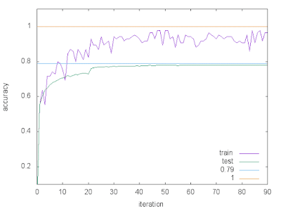
　The CNN model (bvlc_alexnet/bvlc_alexnet.caffemodel) that Caffe provides is fine-tuned on the training dataset. The detailed information on the fine-tuning procedures is described in this page. The prototxt file used for training is as follows: The solver file is as follows: This script is run in order to train the CNN. The fine-tuning process is shown below.

The x-axis indicates the iteration number and the y-axis the recognition accuracy. Because in my work the total iteration number is set to 91,000 and a solver file, where parameters for training are defined, is designed to output the accuracy once per 1000 iterations, the maximum value of the x-axis is 91(=91,000/1000). It can be seen that the recognition accuracy reaches about 77.9%.
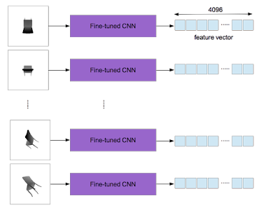
　After training, an output of the layer "fc7" is used as a feature vector (4096 dimensions). In the proposed method a 3D object yields 20 gray images which are converted from depth ones. The fine-tuned CNN used as the feature extractor is applied to each of them and 20 feature vectors are obtained per 3D object.

According to the work by H. Su et al., the element-wise maximum operation across the 20 vectors is used to make a single feature vector with 4096 dimensions as shown below.

It is worthy of noting that one feature vector per 3D object is computed.

Evaluation On SHREC2014

　Now that the feature extractor is constructed, five standard performance metrics, Nearest Neighbor (NN), First-Tier (FT), Second-Tier (ST), F-Measure (F), and Discounted Cumulative Gain (DCG), can be calculated by means of three evaluation programs:

1. SHREC2014_Comprehensive_Evaluation.m
2. SHREC2014_Comprehensive_Evaluation_Proportional_Weight.m
3. SHREC2014_Comprehensive_Evaluation_Reciprocal_Weight.m

These are m-files for MATLAB. The tables shown below compare the results of my method and the previous best results of the other studies which are quoted from the page. I think that there exists a mistake of understanding the F-Measure as the E-Measure in the page.

Performance metrics:

	NN	FT	ST	F	DCG
my result	0.904	0.569	0.683	0.275	0.849
the previous best result	0.868	0.528	0.661	0.255	0.823

Proportional Weighted Performance metrics:

	NN	FT	ST	F	DCG
my result	188.087	123.136	149.292	37.709	179.756
the previous best result	178.981	107.851	144.179	33.691	173.773

Reciprocally Weighted Performance metrics:

	NN	FT	ST	F	DCG
my result	5.025	3.061	3.595	1.820	4.626
the previous best result	4.881	2.905	3.435	1.731	4.470