Mean Shift Filtering 〜Practice by OpenCV〜

in Japanese

Introduction

　In the previous page, I provided a brief explanation of the Mean Shift analysis. In this page, I describe the Mean Shift filtering proposed by D. Comaniciu and P. Meer in [1][2]. I also show the practice of the filtering by the OpenCV library.

Theory

　Suppose we have an $RGB$ image that consists of $n$ pixels each of which has three values $(r,g,b)$. Since the image is regarded as the distribution of the points in the 3-dimensional space, we can define a density function as shown in the previous discussion. We can detect local maximal points of the density by the Mean Shift analysis as illustrated below. In the figure, the blue circles indicate local maximal points.

Any point $\vec{x}$ in the 3-dimensional ($RGB$) space converges toward a local maximal point adjacent to $\vec{x}$. If we replace all points in the image by the corresponding local maximal points, we can accomplish the smoothing of the image. In the above figure, the green line shows the smoothing image.

　It should be noticed that an image has not only color information but also location one. Since the smoothing procedure explained above ignores location information, two distantly-positioned objects that happen to have similar color can be labeled by the same color. When we would like to assign the different labels to them, we cannot employ the procedure. D. Comaniciu and P. Meer expanded the vector $(r,g,b)$ that represents each pixel to the 5-dimensional vector $(x,y,r,g,b)$ which includes location information $(x,y)$^1,2. In this case, the kernel used in the Mean Shift analysis is modified as \begin{equation} K(\vec{x}_i;\;\vec{x},h)=K_{\rm spatial}(\vec{x}_i^{\;s};\;\vec{x}^{\;s},h_s)\;K_{\rm range}(\vec{x}_i^{\;r};\;\vec{x}^{\;r},h_r) \end{equation} where $\vec{x}=(\vec{x}^{\;s},\vec{x}^{\;r})$, $\vec{x}^{\;s}=(x,y)$, $\vec{x}^{\;r}=(r,g,b)$, $h_s$ is the radius of the sphere in the spatial space , and $h_r$ is the the radius of the sphere in the color space. Using the kernel, the mean is calculated by the following expression: \begin{equation} \vec{m}(\vec{x}) = \frac{\sum_{i=1}^{n}\;K(\vec{x}_i;\;\vec{x},h)\;\vec{x}_i}{\sum_{i=1}^{n}\;K(\vec{x}_i;\;\vec{x},h)}. \end{equation} Only when calculating the kernel, $\vec{x}^{\;s}$ and $\vec{x}^{\;r}$ are distinguished. Other calculation is the same as the previous page. Applying the Mean Shift analysis to all points $\{\vec{x}_{i}|i=1,\cdots,n\}$ in the image, we obtain a set of convergence points $\{\vec{z}_{i}|i=1,\cdots,n\}$. By replacing $\vec{x}_i^{\;r}$ (the color component of the original point) by $\vec{z}_i^{\;r}$ (the color component of the convergence point), we generate a new point $\vec{y}_i=(\vec{x}_i^{\;s},\vec{z}_i^{\;r})$. The image constructed from the set $\{\vec{y}_{i}|i=1,\cdots,n\}$ is the final result.

Practice by OpenCV

We can use cv::pyrMeanShiftFiltering. The sample code is as follows: The function cv::pyrMeanShiftFiltering is called in the 14th line. The first argument is an input image, and the second is an output image. The third and fourth arguments are $h_{s}$ and $h_{r}$, respectively. The sixth argument is the termination criteria for the algorithm. If we use pyramid images in the internal calculation, we have to set the level number of them to the fifth argument. Because this time we apply the Mean Shift analysis to the source image only once, we set it to 0. The resultant images are as follows:
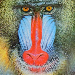
Source Image：

$(h_s,h_r)=(16,32)$:

$(h_s,h_r)=(16,64)$:

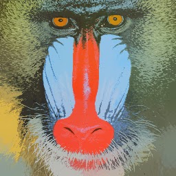
The size of the input image is (256,256) pixels. We set params.max_iteration_count_=30 and params.epsilon_=0.01. Maybe cv::pyrMeanShiftFiltering employs the Fukunaga kernel.

References

1. Mean Shift Analysis and Applications, D. Comaniciu and P. Meer, 1999 (pdf)
2. Mean Shift: A Robust Approach Toward Feature Space Analysis, D. Comaniciu and P. Meer, 2002 (pdf)
3. コンピュータビジョン2 最先端ガイド　第2章, アドコム・メディア株式会社 (in Japanese)